Chapter 6 · Section 4
The Computational Event Horizon and Boundary Information Flow
The physical picture of the event horizon as a computational threshold is set out in Part 2.4; here we give its formal structure.
Computational Event Horizon Architecture
The event horizon represents the critical surface where Pulse amplitude A(r,τ) approaches zero through exponential decay. By examining the Horizon Condition and Pulse Amplitude Decay Equation we can understand how physical processing appears to pass into suspension through event horizon scale where Pulse amplitude approaches zero at Schwarzschild radius representing critical surface for computational state changes, while exponential decay operates through decay length connecting to Pulse Diameter scaling where recursive depth enhancement modifies spatial scales for distance-dependent amplitude reduction from active substrate to event horizon.
Horizon Condition
lim[r→rₛ] A(r,τ) = 0 [∅]
Where:
- lim [∅] - limit operator
- r [𝕃] - radial coordinate
- rₛ [𝕃] - Schwarzschild radius
- A(r,τ) [∅] - Pulse amplitude at radius r and proper time τ
- τ [𝕋] - proper time coordinate
- → [∅] - approaches operator
- 0 [∅] - zero amplitude state
Dimensional analysis:
Where (from the book): 0 [∅], r [𝕃], τ [𝕋]
Read dimensionally: A(r,τ) = 0
[∅]
[∅]
[∅] = [∅] ✓ Valid PulseCore Verified ✓
➢ The Schwarzschild radius r_s = 2GM/c² represents the event horizon scale where physical processing appears to pass into suspension as critical surface where Pulse amplitude approaches zero through exponential decay at event horizon boundary.
Pulse Amplitude Decay Equation
A(r,τ) = A₀ · (1 - exp(-(r-rₛ)/λ)) [∅]
Where:
- A(r,τ) [∅] - Pulse amplitude at radius r and proper time τ
- r [𝕃] - radial coordinate
- τ [𝕋] - proper time coordinate
- A₀ [∅] - Pulse amplitude in the active substrate region, far outside the horizon (r − r_s ≫ λ)
- exp [∅] - exponential function
- rₛ [𝕃] - Schwarzschild radius
- λ [𝕃] - decay length
- PD [𝕃] - Pulse Diameter
- Gℜ(n) [∅] - recursive depth enhancement function
- n [∅] - recursive depth level
Dimensional analysis:
Where (from the book): r [𝕃], τ [𝕋], exp [∅], λ [𝕃], n [∅]
[∅]
[∅] × ([∅] - [∅](([𝕃] - [𝕃]) ÷ [𝕃])) = [∅] × ([∅] - [∅]([𝕃] ÷ [𝕃])) = [∅] × ([∅] - [∅]([∅])) = [∅] × ([∅] - [∅]) = [∅] × [∅] = [∅]
[∅] = [∅] ✓ Valid PulseCore Verified ✓
➢ Decay length connecting to Pulse Diameter scaling through λ = PD · Gℜ(n), where recursive depth enhancement modifies spatial scales enabling exponential decay from active substrate region to event horizon through distance-dependent amplitude reduction.
The Horizon Condition and Pulse Amplitude Decay Equation establish how physical processing appears to pass into suspension through event horizon scale where Pulse amplitude approaches zero at Schwarzschild radius and exponential decay through decay length that connects to Pulse Diameter scaling where recursive depth enhancement modifies spatial scales, demonstrating critical surface where computational processing transitions from active substrate region to suspension state and distance-dependent amplitude reduction from the substrate amplitude A₀ to zero at event horizon through exponential function governed by decay length λ = PD · Gℜ(n).
Causal Influence and Information Flow Cessation
The event horizon marks the computational shell where direct physical causal influence and outward Pulse propagation cease. The data does not stop there: it continues inward, through the rupture at the well's core, and returns by the Data Loop rather than back across the horizon. By examining the Causal Influence Boundary and Information Flow Cessation equation we can understand how computational processing transition operates through Pulse amplitude gradient at event horizon determining causal influence boundary where local Pulse states collapse exponentially toward central Null Well, while information transmission cessation operates through Information Flow Rate reaching zero at Schwarzschild radius where local Pulse states collapse exponentially toward central Null Well via Gravitational Coupling Parameters.
Causal Influence Boundary
∂A/∂r|r=rₛ = A₀/λ [𝕃⁻¹]
Where:
- ∂A/∂r [𝕃⁻¹] - Pulse amplitude gradient with respect to radius
- A [∅] - Pulse amplitude
- r [𝕃] - radial coordinate
- rₛ [𝕃] - Schwarzschild radius
- A₀ [∅] - Pulse amplitude in the active substrate region, far outside the horizon (r − r_s ≫ λ)
- λ [𝕃] - decay length
- | [∅] - evaluation operator at specific point
Dimensional analysis:
Where (from the book): ∂A/∂r [𝕃⁻¹], A [∅], r [𝕃], λ [𝕃]
Read dimensionally: ∂A/∂r = A₀/λ
[𝕃⁻¹]
[∅] ÷ [𝕃] = [𝕃⁻¹]
[𝕃⁻¹] = [𝕃⁻¹] ✓ Valid PulseCore Verified ✓
➢ Beyond this critical surface, local Pulse states collapse exponentially toward the central Null Well through Gravitational Coupling Parameters where Pulse amplitude gradient at event horizon determines causal influence boundary for computational processing transition.
Information Flow Cessation
I⥂(rₛ) = 0 [∅]
Where:
- I⥂(r_s) [∅] - Information Flow Rate at Schwarzschild radius
- rₛ [𝕃] - Schwarzschild radius
- 0 [∅] - zero outward physical flow
Dimensional analysis:
Where (from the book): 0 [∅], I⥂(rₛ) [∅], rₛ [𝕃]
[∅]
[∅]
[∅] = [∅] ✓ Valid PulseCore Verified ✓
➢ Beyond this critical surface, local Pulse states collapse exponentially toward the central Null Well through Gravitational Coupling Parameters where Information Flow Rate reaches zero at Schwarzschild radius marking complete cessation of information transmission across event horizon boundary.
Null Well Formation and Core Dynamics
By examining the Null Well Formation Condition and Mathematical Description of Null Well State we can understand how BPT's reading of singularities operates through critical density threshold for apparent physical suspension where local recursive tension density exceeds the Planck energy density triggering Binary Pulse Cycles compression into sustained zero state, while central physical pause architecture operates through sustained zero state persisting within null well radius after collapse time ensuring existence inside event horizon.
Central Physical Pause Architecture
The Null Well represents the central physical pause point where Binary Pulse Cycles compress into sustained zero state:
- Standard Pulse Cycle: ...0 → 1 → 0 → 1…
- Collapse Sequence: ...0 → 1 → 0 → (collapse) → 0∅
- Null State: 0∅ (physical evolution appears suspended; the data flows on)
Null Well Formation Condition
ℜ⌂ ≥ ρ_P · 𝒞→² = 𝒞→⁷/(ℏG²) [𝕄·𝕃⁻¹·𝕋⁻²]
Where:
- ℜ⌂ [𝕄·𝕃⁻¹·𝕋⁻²] - local recursive tension density
- ρ_P [𝕄·𝕃⁻³] - Planck density, 𝒞→⁵/(ℏG²)
- 𝒞→ [𝕃·𝕋⁻¹] - speed of light
- ℏ [𝕄·𝕃²·𝕋⁻¹] - reduced Planck constant
- G [𝕄⁻¹·𝕃³·𝕋⁻²] - gravitational constant
- ≥ [∅] - greater than or equal to operator
Dimensional analysis:
Where (from the book): ℜ⌂ [𝕄·𝕃⁻¹·𝕋⁻²], ρ_P [𝕄·𝕃⁻³], ℏ [𝕄·𝕃²·𝕋⁻¹], G [𝕄⁻¹·𝕃³·𝕋⁻²]
Read dimensionally: ℜ⌂ ≥ ρ_P · 𝒞→² = 𝒞→⁷/(ℏ × G²)
[𝕄·𝕃⁻¹·𝕋⁻²] ≥ [𝕄·𝕃⁻³] × [𝕃²·𝕋⁻²] = [𝕄·𝕃⁻¹·𝕋⁻²] ≥ [𝕄·𝕃⁻¹·𝕋⁻²]
[𝕃⁷·𝕋⁻⁷] ÷ ([𝕄·𝕃²·𝕋⁻¹] × [𝕄⁻²·𝕃⁶·𝕋⁻⁴]) = [𝕃⁷·𝕋⁻⁷] ÷ [𝕄⁻¹·𝕃⁸·𝕋⁻⁵] = [𝕄·𝕃⁻¹·𝕋⁻²]
[𝕄·𝕃⁻¹·𝕋⁻²] ≥ [𝕄·𝕃⁻¹·𝕋⁻²] = [𝕄·𝕃⁻¹·𝕋⁻²] ✓ Valid PulseCore Verified ✓
➢ Critical density threshold at which physical evolution appears to freeze, reframing singularity physics where local recursive tension density exceeding the Planck energy density triggers Binary Pulse Cycle compression into sustained zero state through central physical pause architecture.
Null Well State
S∅(r < r∅, τ) = 0 ∀τ > τ⦰ [∅]
Where:
- S∅(r < r∅, τ) [∅] - null well state for radius less than null well radius at proper time τ
- r [𝕃] - radial coordinate
- r∅ [𝕃] - Null Well Radius
- τ [𝕋] - proper time coordinate
- τ⦰ [𝕋] - collapse time
- < [∅] - less than operator
- ∀ [∅] - universal quantifier (for all)
- > [∅] - greater than operator
- 0 [∅] - sustained zero state
Dimensional analysis:
Where (from the book): 0 [∅], S∅(r < r∅, τ) [∅], r [𝕃], τ [𝕋], τ⦰ [𝕋]
Read dimensionally: S∅(r < r∅, τ) = 0
[∅]
[∅]
[∅] = [∅] ✓ Valid PulseCore Verified ✓
➢ Ashtekar, Baez, Corichi and Krasnov's quantum geometry findings (Ashtekar, Baez, Corichi & Krasnov, 1998) align with inclusion of Quantum Corrections ensuring the Null Well exists inside the event horizon where sustained zero state persists for all radii within null well radius after collapse time through central physical pause architecture.
The Null Well Formation Condition and Mathematical Description of Null Well State establish how BPT's reading of singularities functions through critical density threshold for apparent physical suspension and central physical pause architecture where local recursive tension density exceeding the Planck energy density triggers Binary Pulse Cycle compression into sustained zero state that persists within null well radius after collapse time, replacing infinite curvature singularities with a finite rupture, where physical evolution appears to stop while the data continues along the new dimension it opens.
This reframes Null Well physics through a Planck density threshold that determines transition from active binary computation to null well state suspension, while Ashtekar, Baez, Corichi and Krasnov's quantum geometry findings (Ashtekar, Baez, Corichi & Krasnov, 1998) align with Quantum Corrections ensuring null well exists inside event horizon through mathematical framework that replaces classical singularity infinities with finite null state architecture.
Universe Genesis and Parameter Modification
By examining the Reactivation Condition, Modified Planck Time, Parameter Modification Framework, and Scaling Function Specifications we can understand how universe genesis operates through accumulated tension exceeding genesis threshold triggering reactivation that launches emergent domains with modified fundamental parameters determined by scaling functions based on collapse properties, while modified Planck time provides temporal quantum for distinct recursive cycles in emergent universes with testable predictions through horizon observables.
Reactivation Mechanisms:
Beyond the Null Well, new recursive Pulse sequences may initiate when boundary conditions satisfy reactivation criteria:
Reactivation Condition
∫◫ σ⫷ dA ≥ T⇌ [𝕄·𝕃²·𝕋⁻²]
Where:
- ∫◫ [∅] - surface integral over boundary
- σ⫷ [𝕄·𝕋⁻²] - accumulated boundary tension per unit area
- dA [𝕃²] - differential area element
- T⇌ [𝕄·𝕃²·𝕋⁻²] - genesis threshold
- ≥ [∅] - greater than or equal to operator
Dimensional analysis:
Where (from the book): ∫◫ [∅], σ⫷ [𝕄·𝕋⁻²], dA [𝕃²], T⇌ [𝕄·𝕃²·𝕋⁻²]
Read dimensionally: σ⫷ × dA ≥ T⇌
[𝕄·𝕋⁻²] × [𝕃²] ≥ [𝕄·𝕃²·𝕋⁻²] = [𝕄·𝕃²·𝕋⁻²] ≥ [𝕄·𝕃²·𝕋⁻²] ✓ Valid PulseCore Verified ✓
➢ The emergent domain launches distinct recursive cycles with modified fundamental parameters when boundary conditions satisfy reactivation criteria through accumulated tension exceeding genesis threshold.
Modified Planck Time
①⥂⧗'⌂ = sqrt(ℏ'G'/𝒞→'⁵) [𝕋]
Where:
- ①⥂⧗'⌂ [𝕋] - modified Pulse Tempo in emergent universe
- ℏ' [𝕄·𝕃²·𝕋⁻¹] - modified reduced Planck constant
- G' [𝕄⁻¹·𝕃³·𝕋⁻²] - modified gravitational constant
- 𝒞→' [𝕃·𝕋⁻¹] - modified speed of light
- sqrt [∅] - square root function
Dimensional analysis:
Where (from the book): G' [𝕄⁻¹·𝕃³·𝕋⁻²]
Read dimensionally: ①⥂⧗'⌂ = sqrt(ℏ'G'/𝒞→'⁵)
[𝕋]
sqrt([𝕄·𝕃²·𝕋⁻¹] × [𝕄⁻¹·𝕃³·𝕋⁻²] ÷ [𝕃⁵·𝕋⁻⁵]) = sqrt([𝕃⁵·𝕋⁻³] ÷ [𝕃⁵·𝕋⁻⁵]) = sqrt([𝕋²]) = [𝕋]
[𝕋] = [𝕋] ✓ Valid PulseCore Verified ✓
➢ Modified Planck time calculated from modified fundamental parameters determines temporal quantum in emergent universe with distinct recursive cycles.
Parameter Modification Framework
ℏ' = ℏ · f₁(M⦰, J, Q) [𝕄·𝕃²·𝕋⁻¹]
Dimensional analysis:
Where (from the book): ℏ [𝕄·𝕃²·𝕋⁻¹], f₁ [∅], M⦰ [𝕄], J [𝕄·𝕃²·𝕋⁻¹], Q [charge], G [𝕄⁻¹·𝕃³·𝕋⁻²], f₂ [∅], ρ⦰ [𝕄·𝕃⁻³], S_S [∅], f₃ [∅], Iℹ [∅]
[𝕄·𝕃²·𝕋⁻¹]
[𝕄·𝕃²·𝕋⁻¹] × [∅]([𝕄], [𝕄·𝕃²·𝕋⁻¹], [charge]) = [𝕄·𝕃²·𝕋⁻¹] × [∅] = [𝕄·𝕃²·𝕋⁻¹]
[𝕄·𝕃²·𝕋⁻¹] = [𝕄·𝕃²·𝕋⁻¹] ✓ Valid PulseCore Verified ✓
G' = G · f₂(ρ⦰, S_S) [𝕄⁻¹·𝕃³·𝕋⁻²]
Dimensional analysis:
[𝕄⁻¹·𝕃³·𝕋⁻²]
[𝕄⁻¹·𝕃³·𝕋⁻²] × [∅]([𝕄·𝕃⁻³], [∅]) = [𝕄⁻¹·𝕃³·𝕋⁻²] × [∅] = [𝕄⁻¹·𝕃³·𝕋⁻²]
[𝕄⁻¹·𝕃³·𝕋⁻²] = [𝕄⁻¹·𝕃³·𝕋⁻²] ✓ Valid PulseCore Verified ✓
𝒞→' = 𝒞→ · f₃(E⧱, Iℹ) [𝕃·𝕋⁻¹]
Where:
- ℏ [𝕄·𝕃²·𝕋⁻¹] - original reduced Planck constant
- f₁ [∅] - scaling function for Planck constant
- M⦰ [𝕄] - collapse mass
- J [𝕄·𝕃²·𝕋⁻¹] - angular momentum
- Q [charge] - electric charge
- G [𝕄⁻¹·𝕃³·𝕋⁻²] - original gravitational constant
- f₂ [∅] - scaling function for gravitational constant
- ρ⦰ [𝕄·𝕃⁻³] - collapse density
- S_S [∅] - entropy
- 𝒞→ [𝕃·𝕋⁻¹] - original speed of light
- f₃ [∅] - scaling function for light speed
- E⧱ [𝕄·𝕃²·𝕋⁻²] - binding energy
- Iℹ [∅] - information content
Dimensional analysis:
Where (from the book): ℏ [𝕄·𝕃²·𝕋⁻¹], f₁ [∅], M⦰ [𝕄], J [𝕄·𝕃²·𝕋⁻¹], Q [charge], G [𝕄⁻¹·𝕃³·𝕋⁻²], f₂ [∅], ρ⦰ [𝕄·𝕃⁻³], S_S [∅], f₃ [∅], Iℹ [∅]
[𝕃·𝕋⁻¹]
[𝕃·𝕋⁻¹] × [∅]([𝕄·𝕃²·𝕋⁻²], [∅]) = [𝕃·𝕋⁻¹] × [∅] = [𝕃·𝕋⁻¹]
[𝕃·𝕋⁻¹] = [𝕃·𝕋⁻¹] ✓ Valid PulseCore Verified ✓
➢ Parameter modification rules determine how fundamental constants change in emergent universes based on collapse mass, angular momentum, charge, density, entropy, binding energy, and information content.
Scaling Function Specifications
f₁(M,J,Q) = (M/M_P)^(-α) · (1 + χ²)^β · (1 + q²)^γ [∅]
Dimensional analysis:
Where (from the book): M [𝕄], J [𝕄·𝕃²·𝕋⁻¹], Q [charge], χ [∅], q [∅], ε₀ [M⁻¹L⁻³T⁴A²], α, [∅], ρ [𝕄·𝕃⁻³], ρ_P [𝕄·𝕃⁻³], S [∅], E [𝕄·𝕃²·𝕋⁻²], I [∅]
[∅]([𝕄], [𝕄·𝕃²·𝕋⁻¹], [charge]) = [∅]
([𝕄] ÷ [𝕄])^([∅]) × ([∅] + [∅])^([∅]) × ([∅] + [∅])^([∅]) = ([𝕄] ÷ [𝕄])^([∅]) × ([∅] + [∅])^([∅]) × ([∅] + [∅])^([∅]) = [∅]^([∅]) × ([∅] + [∅])^([∅]) × ([∅] + [∅])^([∅]) = [∅] × ([∅] + [∅])^([∅]) × ([∅] + [∅])^([∅]) = [∅] × [∅]^([∅]) × ([∅] + [∅])^([∅]) = [∅] × [∅] × ([∅] + [∅])^([∅]) = [∅] × ([∅] + [∅])^([∅]) = [∅] × [∅]^([∅]) = [∅] × [∅] = [∅]
[∅] = [∅] ✓ Valid PulseCore Verified ✓
f₂(ρ,S) = (ρ/ρ_P)^δ · exp(-S/S_BH) [∅]
Dimensional analysis:
Where (from the book): M [𝕄], J [𝕄·𝕃²·𝕋⁻¹], Q [charge], ε₀ [M⁻¹L⁻³T⁴A²], α, [∅], ρ [𝕄·𝕃⁻³], ρ_P [𝕄·𝕃⁻³], S [∅], E [𝕄·𝕃²·𝕋⁻²], I [∅]
[∅]([𝕄·𝕃⁻³], [∅]) = [∅]
([𝕄·𝕃⁻³] ÷ [𝕄·𝕃⁻³])^([∅]) × exp([∅] ÷ [∅]) = [∅]^([∅]) × exp([∅] ÷ [∅]) = [∅] × exp([∅] ÷ [∅]) = [∅] × exp([∅]) = [∅] × [∅] = [∅]
[∅] = [∅] ✓ Valid PulseCore Verified ✓
f₃(E,I) = (E/E_P)^ε · (I/I_P)^ζ [∅]
Where:
- M [𝕄] - mass
- M_P [𝕄] - Planck mass
- J [𝕄·𝕃²·𝕋⁻¹] - angular momentum
- Q [charge] - electric charge
- χ = J𝒞→/(𝒢M²) [∅] - dimensionless spin
- q = Q/(M√(4πε₀𝒢)) [∅] - dimensionless charge
- 𝒞→ [𝕃·𝕋⁻¹] - speed of light
- ε₀ [M⁻¹L⁻³T⁴A²] - permittivity of free space
- α, β, γ, δ, ε, ζ [∅] - exponents determining parameter inheritance
- ρ [𝕄·𝕃⁻³] - density
- ρ_P [𝕄·𝕃⁻³] - Planck density
- S [∅] - entropy
- S_BH [∅] - Bekenstein entropy
- E [𝕄·𝕃²·𝕋⁻²] - energy
- E_P [𝕄·𝕃²·𝕋⁻²] - Planck energy
- I [∅] - information
- I_P [∅] - Planck information
➢ Scaling functions measurable through horizon observables, providing testable BPT predictions where exponents determine parameter inheritance based on mass, angular momentum, charge, density, entropy, binding energy, and information content.
The Reactivation Condition, Modified Planck Time, Parameter Modification Framework, and Scaling Function Specifications establish how universe genesis functions through accumulated tension exceeding genesis threshold that triggers reactivation launching emergent domains with modified fundamental parameters, demonstrating scaling functions based on collapse mass, angular momentum, charge, density, entropy, binding energy, and information content that determine parameter inheritance while modified Planck time calculated from modified constants provides temporal quantum for distinct recursive cycles, enabling testable BPT predictions through horizon observables that measure scaling function effects on fundamental parameter modification in emergent universes.
Information Processing and Computational Load Distribution
Horizon Interface (G) information dynamics: information flowing through the event horizon follows conservation principles. By examining the Information Conservation and Horizon Information Storage equations we can understand how Horizon Interface dynamics operate through information conservation principles where input information equals horizon storage plus transmitted information, while horizon area determines information storage capacity through Planck length scaling with binary encoding factor.
Information Conservation
I_in = I◎ + I⟹ [1ᵇ]
Where:
- I_in [∅] - input information
- I◎ [∅] - horizon information storage
- I⟹ [∅] - transmitted information
Dimensional analysis:
Where (from the book): I_in [1ᵇ], I⟹ [1ᵇ]
[1ᵇ]
[1ᵇ] + [1ᵇ] = [1ᵇ]
[1ᵇ] = [1ᵇ] ✓ Valid PulseCore Verified ✓
➢ Information flows through the event horizon follow conservation principles where input information equals horizon storage plus transmitted information through Horizon Interface (G) dynamics.
Horizon Information Storage
I◎ = A◎/(4 × l_P² · ln(2)) · ℨᵇ [1ᵇ]
Where:
- I◎ [1ᵇ] - horizon information storage, in bits
- A◎ [𝕃²] - horizon area
- l_P [𝕃] - Planck length
- ln 2 [∅] - nats-to-bits conversion, the Binary Information Encoding (G) factor
Dimensional analysis:
Where (from the book): l_P [𝕃]
[1ᵇ]
[𝕃²] ÷ ([∅] × [𝕃²] × [∅]) × [1ᵇ] = [𝕃²] ÷ ([𝕃²] × [∅]) × [1ᵇ] = [𝕃²] ÷ [𝕃²] × [1ᵇ] = [∅] × [1ᵇ] = [1ᵇ]
[1ᵇ] = [1ᵇ] ✓ Valid PulseCore Verified ✓
The Information Conservation and Horizon Information Storage equations establish how Horizon Interface (G) dynamics function through information conservation principles and horizon information storage capacity, demonstrating input information conservation through horizon storage plus transmitted information while horizon area scaled by Planck length and Binary Information Encoding (G) factor determines storage capacity, aligning with 't Hooft and Susskind's holographic principle ('t Hooft, 1993; Susskind, 1995) that incorporates binary substrate structure for computational load distribution across event horizon interface through area-based information encoding mechanisms.
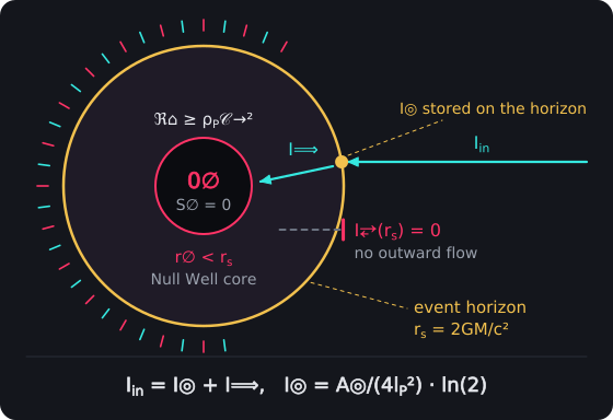
The Computational Event Horizon. Information reaching the horizon at r_s = 2GM/c² is partly stored on it and partly carried inward to the Null Well core, where S∅ = 0. Outward flow at the horizon is zero, I⥂(r_s) = 0, and the balance is I_in = I◎ + I⟹, with I◎ = A◎/(4 l_P² ln 2).
Testable Predictions
The predictions this part shares with Chapter 2 are listed in Part 2.4.
- Parameter correlation measurements: in fundamental constants following f₁, f₂, f₃ scaling functions across cosmic domains, testable through precision spectroscopy of quasar absorption lines with accuracy better than Δα/α ≈ 10⁻⁶.