Chapter 6 · Section 10
Stellar Formalism: The Gas, the Stellar Mass Unit, and the Stellar Null Well
The physical picture of gas, stars and Stellar Null Wells is set out in Part 2.9; here we give its formal structure. Every law below is established by observation and standard astrophysics; what Binary Pulse Theory adds is where each constant comes from: the Planck values of the level (Part 6.5), inherited from the well a universe was born in, and the gas the Physical Nova leaves (Part 3.6). Masses are in kilograms or in Suns (M☉ = 1.989 × 10³⁰ kg), times in seconds or years.
The Data in Matter
Data–Matter Equivalence, Formal G
N⚛ = m_H · c² / (k_B · T · ln(2))
Dimensional analysis:
Where (from the book): m_H [𝕄], c [𝕃·𝕋⁻¹], T [Θ]
[∅]
[𝕄] × [𝕃²·𝕋⁻²] ÷ ([𝕄·𝕃²·𝕋⁻²·Θ⁻¹] × [Θ] × [∅]) = [𝕄·𝕃²·𝕋⁻²] ÷ ([𝕄·𝕃²·𝕋⁻²·Θ⁻¹] × [Θ] × [∅]) = [𝕄·𝕃²·𝕋⁻²] ÷ ([𝕄·𝕃²·𝕋⁻²] × [∅]) = [𝕄·𝕃²·𝕋⁻²] ÷ [𝕄·𝕃²·𝕋⁻²] = [∅]
[∅] = [∅] ✓ Valid PulseCore Verified ✓
A particle's rest energy counted in Landauer bits
Where:
- N⚛ [∅] — bits per hydrogen atom
- m_H [𝕄] — the hydrogen mass, 1.6735 × 10⁻²⁷ kg
- c [𝕃·𝕋⁻¹] — light speed, one Pulse Length a Tempo (ch 1)
- k_B [𝕄·𝕃²·𝕋⁻²·Θ⁻¹] — the Boltzmann constant
- T [Θ] — the temperature of the universe's radiation, T = T⊚/a
➢ With m_H·c² = 1.504 × 10⁻¹⁰ J and k_B·ln 2 = 9.57 × 10⁻²⁴ J/K, N⚛ = 1.57 × 10¹³ K / T. Since T falls as 1/a, N⚛ = N⚛⊚ · a: the data per particle grows in step with the scale factor (Part 3.11), the same growth the Dilation law gives the information of the level.
The Collapse of the Gas
Jeans Length G
λ_J = σ · √(π / (G · ρ))
Dimensional analysis:
Where (from the book): λ_J [𝕃], σ [𝕃·𝕋⁻¹], G [𝕄⁻¹·𝕃³·𝕋⁻²], ρ [𝕄·𝕃⁻³]
[𝕃]
[𝕃·𝕋⁻¹] × √([∅] ÷ ([𝕄⁻¹·𝕃³·𝕋⁻²] × [𝕄·𝕃⁻³])) = [𝕃·𝕋⁻¹] × √([∅] ÷ [𝕋⁻²]) = [𝕃·𝕋⁻¹] × √[𝕋²] = [𝕃·𝕋⁻¹] × [𝕋] = [𝕃]
[𝕃] = [𝕃] ✓ Valid PulseCore Verified ✓
The smallest size at which a region of gas collapses under its own gravity
Where:
- λ_J [𝕃] — the Jeans length
- σ [𝕃·𝕋⁻¹] — the speed of the gas's random motion, its sound speed
- G [𝕄⁻¹·𝕃³·𝕋⁻²] — the universe's gravitational coupling
- ρ [𝕄·𝕃⁻³] — the density of the gas
➢ Below λ_J pressure waves cross the region faster than it can fall in, and it rings instead of collapsing; above it, gravity wins. The Jeans mass of Part 2.9 is the mass of a sphere of diameter λ_J, M_J = (π/6)·ρ·λ_J³, which gives its form (π^(5/2)/6)·σ³/(G^(3/2)·ρ^(1/2)).
Free-Fall Time G
t⇓ = √(3·π / (32 · G · ρ))
Dimensional analysis:
Where (from the book): t⇓ [𝕋], G [𝕄⁻¹·𝕃³·𝕋⁻²], ρ [𝕄·𝕃⁻³]
[𝕋]
√([∅] × [∅] ÷ ([∅] × [𝕄⁻¹·𝕃³·𝕋⁻²] × [𝕄·𝕃⁻³])) = √([∅] ÷ ([∅] × [𝕄⁻¹·𝕃³·𝕋⁻²] × [𝕄·𝕃⁻³])) = √([∅] ÷ ([𝕄⁻¹·𝕃³·𝕋⁻²] × [𝕄·𝕃⁻³])) = √([∅] ÷ [𝕋⁻²]) = √[𝕋²] = [𝕋]
[𝕋] = [𝕋] ✓ Valid PulseCore Verified ✓
How long a cloud takes to collapse with nothing holding it up
Where:
- t⇓ [𝕋] — the free-fall time
- G [𝕄⁻¹·𝕃³·𝕋⁻²] — the universe's gravitational coupling
- ρ [𝕄·𝕃⁻³] — the density of the cloud
➢ It depends on the density alone: a molecular cloud core of 10⁴ molecules a cubic centimetre falls in about 3 × 10⁵ years. This is the clock of star formation, and in this book it is also the clock the game's G is set by, the collapse time of the universe's own matter (Part 3.10, the Rupture Rule).
Star Formation Rate G
Ṁ⊛ = ε⇓ · M_gas / t⇓
Dimensional analysis:
Where (from the book): Ṁ⊛ [𝕄·𝕋⁻¹], ε⇓ [∅], M_gas [𝕄], t⇓ [𝕋]
[𝕄·𝕋⁻¹]
[∅] × [𝕄] ÷ [𝕋] = [𝕄] ÷ [𝕋] = [𝕄·𝕋⁻¹]
[𝕄·𝕋⁻¹] = [𝕄·𝕋⁻¹] ✓ Valid PulseCore Verified ✓
Gas turns into stars at about one percent of its mass per free-fall time
Where:
- Ṁ⊛ [𝕄·𝕋⁻¹] — the rate gas becomes stars
- ε⇓ [∅] — the efficiency per free-fall time, ≈ 0.01 (Krumholz & McKee, 2005)
- M_gas [𝕄] — the mass of dense gas
- t⇓ [𝕋] — the free-fall time
➢ The efficiency is low because stars push back: their light, winds and supernovae heat and disperse the gas that would form more of them. A universe therefore turns its gas into stars slowly, over many free-fall times, and the gas left over is what its later generations, and its Null Wells, draw on.
Gas Depletion Law G
t⇣⊛ = t⇣⊚ · (ρ / ρ⇥)^(−0.4)
Dimensional analysis:
Where (from the book): t⇣⊛ [𝕋], t⇣⊚ [𝕋], ρ [𝕄·𝕃⁻³], ρ⇥ [𝕄·𝕃⁻³]
[𝕋]
[𝕋] × ([𝕄·𝕃⁻³] ÷ [𝕄·𝕃⁻³])^([∅]) = [𝕋] × ([𝕄·𝕃⁻³] ÷ [𝕄·𝕃⁻³])^([∅]) = [𝕋] × [∅]^([∅]) = [𝕋] × [∅] = [𝕋]
[𝕋] = [𝕋] ✓ Valid PulseCore Verified ✓
Gas in galaxies turns into stars over a depletion time, shorter where it is denser
Where:
- t⇣⊛ [𝕋] — the time a region takes to turn its gas into stars at its present rate
- t⇣⊚ [𝕋] — the depletion time at the threshold density: about 2 × 10⁹ years in galaxies today, about 0.145 of the universe's age
- ρ [𝕄·𝕃⁻³] — the density of the gas
- ρ⇥ [𝕄·𝕃⁻³] — the threshold above which gas forms stars
➢ The Kennicutt–Schmidt law (Kennicutt, 1998; Bigiel et al., 2008), written as a depletion time: the star formation rate per area rises as the gas per area to the 1.4, so the time to use the gas falls as its −0.4. It is the rule every cosmological simulation uses below the scale it can resolve, since no simulation of a universe resolves the cores where stars actually form. Measured over the whole life of a universe, the depletion time is a fixed share of its age.
Depletion Time Evolution G
t⇣⊚(a) = t⇣⊚ · a^(0.6)
Dimensional analysis:
Where (from the book): t⇣⊚(a) [𝕋], t⇣⊚ [𝕋], a [∅]
[𝕋]
[𝕋] × [∅]^([∅]) = [𝕋] × [∅]^([∅]) = [𝕋] × [∅] = [𝕋]
[𝕋] = [𝕋] ✓ Valid PulseCore Verified ✓
Galaxies used their gas faster when the universe was young: the depletion time grows with the scale factor
Where:
- t⇣⊚(a) [𝕋] — the depletion time at the threshold density when the scale factor is a
- t⇣⊚ [𝕋] — its value at full size, a = 1: about 2 × 10⁹ years, 0.145 of the life
- a [∅] — the scale factor, 1 at the End of the Outward Expansion
➢ The molecular gas of galaxies on the main sequence is used over a time that scales as (1 + z)^(−0.6): about 0.7 billion years at cosmic noon against 2 billion today (Genzel et al., 2015; Tacconi et al., 2018). With 1 + z = 1/a the law reads a^0.6. It is why the star formation of a universe peaks early and falls: its galaxies burn their gas fastest while it is young and plentiful, near a quarter of the life (cosmic noon, z ≈ 2, Madau & Dickinson, 2014), and by the End of the Outward Expansion form stars at about an eighth of that rate, the gas used and the little left used slowly. The game applies it to every cloud (stars.js), so the life of a universe shows the sky's rise and fall.
The Stellar Mass Unit
Planck Mass of a Level G
m_P = √(ħ · c / G)
Dimensional analysis:
Where (from the book): m_P [𝕄], ħ [𝕄·𝕃²·𝕋⁻¹], c [𝕃·𝕋⁻¹], G [𝕄⁻¹·𝕃³·𝕋⁻²]
[𝕄]
√([𝕄·𝕃²·𝕋⁻¹] × [𝕃·𝕋⁻¹] ÷ [𝕄⁻¹·𝕃³·𝕋⁻²]) = √([𝕄·𝕃³·𝕋⁻²] ÷ [𝕄⁻¹·𝕃³·𝕋⁻²]) = √[𝕄²] = [𝕄]
[𝕄] = [𝕄] ✓ Valid PulseCore Verified ✓
The mass of one Pulse at the level, built from its Planck constant, light speed and gravity
Where:
- m_P [𝕄] — the Planck mass, 2.176 × 10⁻⁸ kg in our universe
- ħ [𝕄·𝕃²·𝕋⁻¹] — the reduced Planck constant of the level (Part 2.5)
- c [𝕃·𝕋⁻¹] — light speed, one Pulse Length a Tempo (ch 1)
- G [𝕄⁻¹·𝕃³·𝕋⁻²] — the universe's gravitational coupling
➢ In this book ħ, and with it the Planck mass, is a constant of the level, set at genesis by the well (Part 6.5, Density and the Relative Planck Constant). Every stellar quantity below carries m_P, and so carries the lineage.
Stellar Mass Unit, Formal G
M⋆ = (m_P / m_H)² · m_P
Dimensional analysis:
Where (from the book): M⋆ [𝕄], m_P [𝕄], m_H [𝕄], ħ [𝕄·𝕃²·𝕋⁻¹], c [𝕃·𝕋⁻¹], G [𝕄⁻¹·𝕃³·𝕋⁻²]
[𝕄]
([𝕄] ÷ [𝕄])² × [𝕄] = [∅]² × [𝕄] = [∅] × [𝕄] = [𝕄]
[𝕄] = [𝕄] ✓ Valid PulseCore Verified ✓
The one mass every star, limit and remnant is a multiple of
Where:
- M⋆ [𝕄] — the Stellar Mass Unit: 3.68 × 10³⁰ kg = 1.85 M☉ in our universe
- m_P [𝕄] — the Planck mass of the level
- m_H [𝕄] — the hydrogen mass, 1.6735 × 10⁻²⁷ kg
- ħ [𝕄·𝕃²·𝕋⁻¹] — the reduced Planck constant of the level (Part 2.5)
- c [𝕃·𝕋⁻¹] — light speed, one Pulse Length a Tempo (ch 1)
- G [𝕄⁻¹·𝕃³·𝕋⁻²] — the universe's gravitational coupling
➢ A star in balance has its gravity held off by pressure; its central temperature must reach fusion, its electrons must not yet be crushed together, and its own light must not blow it apart. Each of those conditions sets its mass within a factor of order unity of M⋆ (Carr & Rees, 1979): the hydrogen-burning limit ≈ 0.04 M⋆, the Chandrasekhar limit ≈ 0.77 M⋆, the most massive stable stars ≈ 50 – 100 M⋆. The ratio m_P/m_H ≈ 1.3 × 10¹⁹ is why a star holds about 10⁵⁷ atoms.
Solar Mass of a Universe G
M☉(u) ≈ 0.54 · M⋆(u)
Dimensional analysis:
Where (from the book): M☉(u) [𝕄], M⋆(u) [𝕄]
[𝕄] ≈ [∅] × [𝕄] = [𝕄] ≈ [𝕄] ✓ Valid PulseCore Verified ✓
Each universe's own Sun, a fixed share of its Stellar Mass Unit
Where:
- M☉(u) [𝕄] — the mass of a Sun-like star in universe u
- M⋆(u) [𝕄] — that universe's Stellar Mass Unit, from its own Planck values
➢ Our Sun is 0.54 of our Stellar Mass Unit. A universe born of a different well, with a different ħ and so a different m_P, has a Sun of a different mass, and its whole stellar sequence (its red dwarfs, its supernova threshold, its Stellar Null Wells) moves with it, in the same proportions.
Stars in Balance
Mass–Luminosity Relation G
L⊛ = L☉ · (M/M☉)^(3.5)
Dimensional analysis:
Where (from the book): L⊛ [𝕄·𝕃²·𝕋⁻³], L☉ [𝕄·𝕃²·𝕋⁻³], M [𝕄], M☉ [𝕄]
[𝕄·𝕃²·𝕋⁻³]
[𝕄·𝕃²·𝕋⁻³] × ([𝕄] ÷ [𝕄])^([∅]) = [𝕄·𝕃²·𝕋⁻³] × ([𝕄] ÷ [𝕄])^([∅]) = [𝕄·𝕃²·𝕋⁻³] × [∅]^([∅]) = [𝕄·𝕃²·𝕋⁻³] × [∅] = [𝕄·𝕃²·𝕋⁻³]
[𝕄·𝕃²·𝕋⁻³] = [𝕄·𝕃²·𝕋⁻³] ✓ Valid PulseCore Verified ✓
A star's brightness rises steeply with its mass
Where:
- L⊛ [𝕄·𝕃²·𝕋⁻³] — the luminosity of a main-sequence star
- L☉ [𝕄·𝕃²·𝕋⁻³] — the Sun's, 3.828 × 10²⁶ W
- M [𝕄] — the star's mass
- M☉ [𝕄] — the mass of the Sun
➢ The exponent runs from about 2.3 for red dwarfs to about 4 near a Sun, and falls toward 1 for the heaviest stars, which shine close to their Eddington limit; 3.5 is the average over the stars that matter most for the light of a galaxy.
Main-Sequence Lifetime, Formal G
τ⊛ = ε⊛ · f⊛ · M · c² / L⊛
Dimensional analysis:
Where (from the book): τ⊛ [𝕋], ε⊛ [∅], f⊛ [∅], M [𝕄], c [𝕃·𝕋⁻¹], L⊛ [𝕄·𝕃²·𝕋⁻³]
[𝕋]
[∅] × [∅] × [𝕄] × [𝕃²·𝕋⁻²] ÷ [𝕄·𝕃²·𝕋⁻³] = [∅] × [𝕄] × [𝕃²·𝕋⁻²] ÷ [𝕄·𝕃²·𝕋⁻³] = [𝕄] × [𝕃²·𝕋⁻²] ÷ [𝕄·𝕃²·𝕋⁻³] = [𝕄·𝕃²·𝕋⁻²] ÷ [𝕄·𝕃²·𝕋⁻³] = [𝕋]
[𝕋] = [𝕋] ✓ Valid PulseCore Verified ✓
A star lives as long as the fuel in its core lasts at the rate it shines
Where:
- τ⊛ [𝕋] — the main-sequence lifetime
- ε⊛ [∅] — the share of rest mass hydrogen fusion releases, 0.007
- f⊛ [∅] — the share of the star's hydrogen its core burns, ≈ 0.1
- M [𝕄] — the star's mass
- c [𝕃·𝕋⁻¹] — light speed, one Pulse Length a Tempo (ch 1)
- L⊛ [𝕄·𝕃²·𝕋⁻³] — its luminosity
➢ For the Sun this gives 1.04 × 10¹⁰ years. With L⊛ ∝ M^3.5 it gives τ⊛ ∝ M^(−2.5), the law of Part 2.9: the fuel grows as the mass and the burning as its 3.5th power.
Eddington Luminosity G
L⇑ = 4 · π · G · M · m_H · c / σ⊤
Dimensional analysis:
Where (from the book): L⇑ [𝕄·𝕃²·𝕋⁻³], G [𝕄⁻¹·𝕃³·𝕋⁻²], M [𝕄], m_H [𝕄], c [𝕃·𝕋⁻¹], σ⊤ [𝕃²]
[𝕄·𝕃²·𝕋⁻³]
[∅] × [∅] × [𝕄⁻¹·𝕃³·𝕋⁻²] × [𝕄] × [𝕄] × [𝕃·𝕋⁻¹] ÷ [𝕃²] = [∅] × [𝕄⁻¹·𝕃³·𝕋⁻²] × [𝕄] × [𝕄] × [𝕃·𝕋⁻¹] ÷ [𝕃²] = [𝕄⁻¹·𝕃³·𝕋⁻²] × [𝕄] × [𝕄] × [𝕃·𝕋⁻¹] ÷ [𝕃²] = [𝕃³·𝕋⁻²] × [𝕄] × [𝕃·𝕋⁻¹] ÷ [𝕃²] = [𝕄·𝕃³·𝕋⁻²] × [𝕃·𝕋⁻¹] ÷ [𝕃²] = [𝕄·𝕃⁴·𝕋⁻³] ÷ [𝕃²] = [𝕄·𝕃²·𝕋⁻³]
[𝕄·𝕃²·𝕋⁻³] = [𝕄·𝕃²·𝕋⁻³] ✓ Valid PulseCore Verified ✓
The brightest a body of mass M can shine before its light pushes its own matter away
Where:
- L⇑ [𝕄·𝕃²·𝕋⁻³] — the Eddington luminosity, 1.26 × 10³¹ W per solar mass
- G [𝕄⁻¹·𝕃³·𝕋⁻²] — the universe's gravitational coupling
- M [𝕄] — the mass of the star or Null Well
- m_H [𝕄] — the hydrogen mass
- c [𝕃·𝕋⁻¹] — light speed, one Pulse Length a Tempo (ch 1)
- σ⊤ [𝕃²] — the Thomson cross-section of the electron, 6.652 × 10⁻²⁹ m²
➢ It caps the mass of stars, since the heaviest would outshine their own gravity, and it caps how fast a Null Well can accrete, since the matter falling in shines as it falls.
The Ends of Stars
Chandrasekhar Limit, Formal G
M⊘ = 3.098 · m_P³ / (μₑ · m_H)²
Dimensional analysis:
Where (from the book): M⊘ [𝕄], m_P [𝕄], μₑ [∅], ħ [𝕄·𝕃²·𝕋⁻¹], c [𝕃·𝕋⁻¹], G [𝕄⁻¹·𝕃³·𝕋⁻²], m_H [𝕄]
[𝕄]
[∅] × [𝕄³] ÷ ([∅] × [𝕄])² = [𝕄³] ÷ ([∅] × [𝕄])² = [𝕄³] ÷ [𝕄]² = [𝕄³] ÷ [𝕄²] = [𝕄]
[𝕄] = [𝕄] ✓ Valid PulseCore Verified ✓
The heaviest a white dwarf can be: electron pressure holds no more
Where:
- M⊘ [𝕄] — the Chandrasekhar mass, 1.43 M☉ for a carbon–oxygen white dwarf
- m_P [𝕄] — the Planck mass of the level, √(ħ·c/G)
- μₑ [∅] — the mass per electron in units of m_H, 2 for carbon and oxygen
- ħ [𝕄·𝕃²·𝕋⁻¹] — the reduced Planck constant of the level (Part 2.5)
- c [𝕃·𝕋⁻¹] — light speed, one Pulse Length a Tempo (ch 1)
- G [𝕄⁻¹·𝕃³·𝕋⁻²] — the universe's gravitational coupling
- m_H [𝕄] — the hydrogen mass
➢ It is M⋆ times 3.098/μₑ², about 0.77 M⋆: a pure ratio of the Pulse to the matter quantum. A dead core below it settles as a white dwarf; one above it collapses on, to a neutron star or a Stellar Null Well.
White Dwarf Initial–Final Mass Relation G
M⊘f ≈ 0.109 · M + 0.394 · M☉
Dimensional analysis:
Where (from the book): M⊘f [𝕄], M [𝕄], M☉ [𝕄]
[𝕄] ≈ [∅] × [𝕄] + [∅] × [𝕄] = [𝕄] ≈ [𝕄] + [∅] × [𝕄] = [𝕄] ≈ [𝕄] + [𝕄] = [𝕄] ≈ [𝕄] ✓ Valid PulseCore Verified ✓
The white dwarf a star leaves, from its birth mass
Where:
- M⊘f [𝕄] — the white dwarf's mass
- M [𝕄] — the star's birth mass, 0.8 – 8 M☉
- M☉ [𝕄] — the mass of the Sun
➢ From white dwarfs in star clusters of known age (Kalirai et al., 2008). A Sun leaves about 0.5 M☉; a star of 8 M☉ leaves about 1.3, just under the limit. The rest of the star is returned to the gas, enriched.
Stellar Null Well Threshold G
M▣ > M_TOV
Dimensional analysis:
Where (from the book): M▣ [𝕄], M_TOV [𝕄]
[𝕄] > [𝕄] ✓ Valid PulseCore Verified ✓
A dead core heavier than any neutron star can be, M_TOV ≈ 2.3 M☉, becomes a Null Well
Where:
- M▣ [𝕄] — the mass of the collapsed core
- M_TOV [𝕄] — the Tolman–Oppenheimer–Volkoff limit, 2.1 – 2.3 M☉ by the heaviest neutron stars observed
➢ With the neutron-star equation of state still uncertain, the limit is taken from observation. Cores above it meet the Null Well Formation Condition (Part 6.2): recursion at the core passes the Zinf-scaled critical threshold and the region goes to physical silence behind a horizon r▣ = 2GM▣/c².
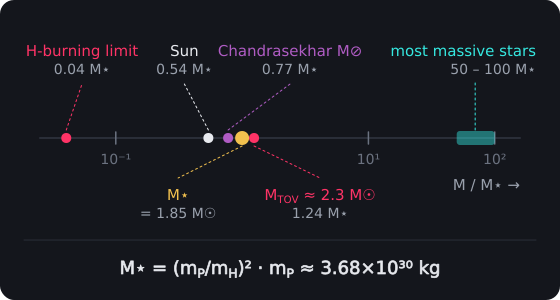
The Stellar Mass Unit. Every stellar mass scale is a multiple of M⋆ = (m_P/m_H)² · m_P ≈ 3.68 × 10³⁰ kg ≈ 1.85 M☉: the hydrogen-burning limit at 0.04 M⋆, the Sun at 0.54 M⋆, the Chandrasekhar limit at 3.098/μₑ² ≈ 0.77 M⋆ and the most massive stars at 50–100 M⋆. Beyond the neutron-star limit M_TOV ≈ 2.3 M☉ ≈ 1.24 M⋆ a dead core becomes a Stellar Null Well.
Stellar Null Well Fraction G
f▣ = N_well / N⊛
Dimensional analysis:
Where (from the book): f▣ [∅], N_well [∅], N⊛ [∅], M▣⁰ [𝕄], M⇓ [𝕄], M⇑ [𝕄], dN/dM [𝕄⁻¹]
[∅]
[∅] ÷ [∅] = [∅]
[∅] = [∅] ✓ Valid PulseCore Verified ✓
The share of all stars that end as Stellar Null Wells
Where:
- f▣ [∅] — the fraction of stars born that end as Null Wells, ≈ 1.3 – 1.8 × 10⁻³ for the Kroupa Initial Mass Function
- N_well [∅] — the stars born between M▣⁰ and M⇑, the integral of dN/dM over those masses
- N⊛ [∅] — all the stars born, the integral of dN/dM from M⇓ to M⇑
- M▣⁰ [𝕄] — the lowest birth mass that leaves a Null Well, ≈ 20 – 25 M☉
- M⇓ [𝕄] — the hydrogen-burning limit, 0.075 M☉
- M⇑ [𝕄] — the most massive stars, ≈ 150 M☉
- dN/dM [𝕄⁻¹] — the Initial Mass Function (Part 2.9)
➢ About one star in six hundred. By the same integral, 76 percent of stars are red dwarfs and 0.6 percent end in core-collapse supernovae.
The Stellar Null Well After Birth
Eddington Growth Time G
t⇑ = ε⇑ · σ⊤ · c / (4 · π · G · m_H · (1 − ε⇑))
Dimensional analysis:
Where (from the book): t⇑ [𝕋], ε⇑ [∅], σ⊤ [𝕃²], c [𝕃·𝕋⁻¹], G [𝕄⁻¹·𝕃³·𝕋⁻²], m_H [𝕄]
[𝕋]
[∅] × [𝕃²] × [𝕃·𝕋⁻¹] ÷ ([∅] × [∅] × [𝕄⁻¹·𝕃³·𝕋⁻²] × [𝕄] × ([∅] - [∅])) = [𝕃²] × [𝕃·𝕋⁻¹] ÷ ([∅] × [∅] × [𝕄⁻¹·𝕃³·𝕋⁻²] × [𝕄] × ([∅] - [∅])) = [𝕃³·𝕋⁻¹] ÷ ([∅] × [∅] × [𝕄⁻¹·𝕃³·𝕋⁻²] × [𝕄] × ([∅] - [∅])) = [𝕃³·𝕋⁻¹] ÷ ([∅] × [𝕄⁻¹·𝕃³·𝕋⁻²] × [𝕄] × ([∅] - [∅])) = [𝕃³·𝕋⁻¹] ÷ ([𝕄⁻¹·𝕃³·𝕋⁻²] × [𝕄] × ([∅] - [∅])) = [𝕃³·𝕋⁻¹] ÷ ([𝕃³·𝕋⁻²] × ([∅] - [∅])) = [𝕃³·𝕋⁻¹] ÷ ([𝕃³·𝕋⁻²] × [∅]) = [𝕃³·𝕋⁻¹] ÷ [𝕃³·𝕋⁻²] = [𝕋]
[𝕋] = [𝕋] ✓ Valid PulseCore Verified ✓
The fastest a Null Well can grow by accretion: e-folding its mass in this time
Where:
- t⇑ [𝕋] — the Salpeter time, ≈ 5 × 10⁷ years
- ε⇑ [∅] — the share of infalling rest mass radiated away, ≈ 0.1
- σ⊤ [𝕃²] — the Thomson cross-section
- c [𝕃·𝕋⁻¹] — light speed, one Pulse Length a Tempo (ch 1)
- G [𝕄⁻¹·𝕃³·𝕋⁻²] — the universe's gravitational coupling
- m_H [𝕄] — the hydrogen mass
➢ A well accreting at its Eddington limit grows as e^(t/t⇑), independent of its mass. A 100 M☉ Population III seed reaches 10⁹ M☉ in about 0.8 × 10⁹ years only if it accretes at the limit without pause, which is why the giant Null Wells already present in the first billion years require early, heavy seeds, mergers, or both.
Hawking Lifetime G
t⇣ = 5120 · π · G² · M³ / (ħ · c⁴)
Dimensional analysis:
Where (from the book): t⇣ [𝕋], G [𝕄⁻¹·𝕃³·𝕋⁻²], M [𝕄], ħ [𝕄·𝕃²·𝕋⁻¹], c [𝕃·𝕋⁻¹]
[𝕋]
[∅] × [∅] × [𝕄⁻²·𝕃⁶·𝕋⁻⁴] × [𝕄³] ÷ ([𝕄·𝕃²·𝕋⁻¹] × [𝕃⁴·𝕋⁻⁴]) = [∅] × [𝕄⁻²·𝕃⁶·𝕋⁻⁴] × [𝕄³] ÷ ([𝕄·𝕃²·𝕋⁻¹] × [𝕃⁴·𝕋⁻⁴]) = [𝕄⁻²·𝕃⁶·𝕋⁻⁴] × [𝕄³] ÷ ([𝕄·𝕃²·𝕋⁻¹] × [𝕃⁴·𝕋⁻⁴]) = [𝕄·𝕃⁶·𝕋⁻⁴] ÷ ([𝕄·𝕃²·𝕋⁻¹] × [𝕃⁴·𝕋⁻⁴]) = [𝕄·𝕃⁶·𝕋⁻⁴] ÷ [𝕄·𝕃⁶·𝕋⁻⁵] = [𝕋]
[𝕋] = [𝕋] ✓ Valid PulseCore Verified ✓
How long a Null Well with nothing to eat takes to evaporate
Where:
- t⇣ [𝕋] — the evaporation time
- G [𝕄⁻¹·𝕃³·𝕋⁻²] — the universe's gravitational coupling
- M [𝕄] — the mass of the Null Well
- ħ [𝕄·𝕃²·𝕋⁻¹] — the reduced Planck constant of the level (Part 2.5)
- c [𝕃·𝕋⁻¹] — light speed, one Pulse Length a Tempo (ch 1)
➢ For one Sun, 2.1 × 10⁶⁷ years; it grows as M³, so the lightest evaporate first and each quickens at its end. Evaporation is the last way a Null Well returns its data to the Source (Part 3.10); for a well in our universe it begins in earnest only when the universe around it is colder than the well, long after the last stars.
The Galaxies a Universe Holds
The Null Well Progeny Count Law (Part 2.7) counts every well a universe forms, and stellar wells are the bulk of that census (Part 2.3), so it is not a count of galaxies. The number of galaxies is its own quantity, which Part 3.13 already relates to it: a galaxy like ours holds 2^(L/3) divided by the number of galaxies in stellar wells. What sets that number is cooling. Gas falling into a halo is heated to its virial temperature and goes on into stars only if it radiates that heat within a free-fall time (Rees & Ostriker, 1977; Silk, 1977; White & Rees, 1978). Above a certain mass it cannot. That mass is the knee of the galaxy mass function: below it galaxies are many, above it they grow rare.
Cooling Mass G
t⊹(T_v(M_c), n_H) = t_ff [𝕋]
Dimensional analysis:
Where (from the book): t⊹ [𝕋], T_v [Θ], M_c [𝕄], n_H [𝕃⁻³], t_ff [𝕋]
[𝕋]([Θ]([𝕄]), [𝕃⁻³]) = [𝕋]([Θ], [𝕃⁻³]) = [𝕋]
[𝕋]
[𝕋] = [𝕋] ✓ Valid PulseCore Verified ✓
The halo mass whose gas cools in exactly a free-fall time; above it a halo’s gas stays hot
Where:
- M_c [𝕄] — the cooling mass
- t⊹ [𝕋] — the cooling time, (3/2)(n_e + n_t) k_B T / (n_e n_t n_H Λ_N), with the cooling function of Sutherland & Dopita (1993) at the gas’s metals
- T_v(M) [Θ] — the virial temperature, μ m_p v_c² / (2 k_B), with v_c ≈ 100 km/s · (M / 10¹² M☉)^(1/3) · a^(−1/2), a halo being denser the smaller the universe
- n_H [𝕃⁻³] — the halo’s hydrogen density, 200 times the mean at that time
- t_ff [𝕋] — the free-fall time at 200 times the mean matter density
➢ With the game’s own cooling tables the cooling mass is 1.0 to 2.4 × 10¹² Suns of halo through the life, at metals a tenth to a third of the Sun’s, its gas at 0.6 to 2.8 million kelvin. It is the halo mass at which galaxies turn their gas into stars most efficiently, measured near 10¹² Suns (Behroozi, Wechsler & Conroy, 2013), whose galaxies sit at the knee of the stellar mass function, about 4.6 × 10¹⁰ Suns of stars (Part 3.14).
Galaxy Count from Cooling G
N⦾ = M_h / (κ_S × M_c) [∅]
Dimensional analysis:
Where (from the book): N⦾ [∅], M_h [𝕄], κ_S [∅], M_c [𝕄]
[∅]
[𝕄] ÷ ([∅] × [𝕄]) = [𝕄] ÷ [𝕄] = [∅]
[∅] = [∅] ✓ Valid PulseCore Verified ✓
The universe’s matter in halos, over the mean galaxy’s halo, which the cooling mass sets
Where:
- N⦾ [∅] — the number of galaxies the universe holds
- M_h [𝕄] — the matter in its halos, its matter and its Data Matter together
- κ_S [∅] — the mean galaxy’s halo over the cooling mass, for a Schechter distribution of slope α ≈ −1.2 down to the filtering mass M_F ≈ 10⁹ Suns: Γ(α + 2) / Γ(α + 1, M_F / M_c) ≈ 0.08 (Schechter, 1976)
- M_c [𝕄] — the cooling mass (above)
➢ For the matter of our observable universe, about 5 × 10²³ Suns with its dark matter, it gives about 4 × 10¹² galaxies, against the measured estimate of about 2 × 10¹² (Conselice et al., 2016). Divided into the Progeny Count it leaves about 5 × 10⁷ stellar wells a galaxy, near the 10⁸ to 10⁹ of Part 3.13. The law is a candidate: it takes the cooling mass to be the knee, the standard reading in astronomy, and nothing else beyond the book’s own laws.
In the game. A drawn galaxy stands for N⦾ divided by the galaxies drawn, so its real halo is its share of the matter over that. From that real halo come its virial temperature and its cooling (Part 3.12). While halos are small and the universe dense, their gas cools and star formation rises. As halos grow past the cooling mass and the universe thins, their gas stays hot, the wells that feed in them keep it hot, and star formation falls. The rise and fall come from these laws, not from a curve set in the game.
The Game's Reading, Formally
The simulation cannot reach the scale at which m_P and m_H are separate numbers: its cells are Pulse Lengths and its matter is counted in bits, so its universes are ratios of ours. It keeps every law above in its proportions. The gas is the matter the Physical Nova condenses; ρ is its mass per cell, σ the spread of its velocities about their local mean. At the game's scale the Pulse and the matter quantum are one cell each, m_P = m_H, so M⋆ = 1 cell and the game's Sun is M☉(game) = 0.54 cells by the Solar Mass of a Universe. The game cannot resolve the cores where stars form, so it forms them as cosmological simulations do, by the Gas Depletion Law: gas in 8 × 8-cell clouds denser than twice the mean (per real area of the torus) turns into stars over t⇣⊛ = 0.145 · T · (ρ/ρ⇥)^(−0.4), T the life from the Physical Nova, each star drawing its mass from its cloud's gas. Every mass then reads in those Suns, and the type, colour, luminosity (M^3.5), lifetime (M^(−2.5), the game's Sun living a set share of its universe's life), end and remnant follow the tables of Part 2.9. Only a core past the neutron-star limit becomes a well: a Stellar Null Well, born small, growing at most at its Eddington rate, merging, and evaporating by Hawking radiation (ħ = 1 in the game's units) when starved.
6.10 Testable Predictions
- Every stellar mass scale is a multiple of m_P³/m_H²: the hydrogen-burning limit, the Chandrasekhar limit and the most massive stars stand in fixed ratios (0.04 : 0.77 : 50 – 100) in every universe, whatever its Planck values
- The fraction of stars that end as Stellar Null Wells, f▣ ≈ 1.5 × 10⁻³, together with the history of star formation, accounts for the bulk of the Null Well census N(L) = 2^(L/3)
- The giant Null Wells of the first billion years grew from heavy seeds (Population III remnants or direct collapse) and mergers, since single light seeds cannot reach them at the Eddington rate
- No Null Well forms from a single star between about 50 and 130 M☉; those observed there were assembled by mergers
Chapter 6 Review
This review gathers what each part of the chapter formalizes. The physical picture behind it, and the predictions it shares with Chapter 2, are set out in the Chapter 2 Review.
Key Developments
Modified Constants Framework
The Key Math opens the chapter with the Dimensional Consistency Constraint α²·β⁵ = γ·δ, which binds a child universe’s Planck time, light speed, gravity and quantum of action so that its Planck time is still √(ℏG/c⁵), and with the Inherited Planck Time ①⥂⧗'⌂ = ①⥂⧗♁ × (M∅ / M_P)^(1/2), set by the Null Mass of the collapse that made it.
Temporal Quantization
Part 6.2 writes the Planck Pulse as the complete cycle 0 → 1 → 0 with period ①⥂⧗♁, giving the Planck frequency ν_P = 1/①⥂⧗♁, the energy quantum E_P = ℏ/t_P and the discrete interval Δt = n·①⥂⧗♁.
Null Well Formation Dynamics
Parts 6.2–6.4 set the formation condition ℜ♁(x,τ) ≥ ℜρ⨶ = k × ρ_P × 𝒞→², the collapse evolution dℜ/dτ = -γℜ² + σ∇²ℜ, and the horizon condition lim[r→r_s] A(r,τ) = 0 with A(r,τ) = A₀ · (1 - exp(-(r-r_s)/λ)). Part 6.7 adds the collapse trajectory and its time scale τ⦰.
Genesis Reactivation Mechanisms
Reactivation is the threshold T⫷ ≥ T⇌ (Part 6.7), with T⇌ = k⇌ · S_c · ρ_P · 𝒞→² · l_P³ at the boundary (Parts 6.3 and 6.7). Part 6.6 gives the genesis sequence and its bifurcation condition ∂²S/∂τ² |_τ=0 = δ(M_n - M⨶), and Part 6.7 the genesis function G[0∅].
Density-Dependent Constants
Part 6.5 makes the Pulse Tempo local, ①⥂⧗'⌂ = ①⥂⧗⌂ · fρ(ρ⦰) with fρ(ρ) = (ρ_P/ρ⦰)^(1/2), and binds the modified constants through g₁(ρ) · g₂(ρ) = g₃(ρ)⁵ · (ρ_P/ρ⦰) and α + β − 5γ = 1, so the Pulse time scales as √(g₁g₂/g₃⁵) = (ρ_P/ρ⦰)^½. Part 6.6 writes the same scaling through Null Mass, ①⥂⧗'⌂ = ①⥂⧗⌂ · (M_n/M_P)^(1/2).
Information Conservation Across Transitions
Part 6.4 balances information at the horizon, I_in = I◎ + I⟹, with storage I◎ = A◎/(4 l_P² · ln(2)) · ℨᵇ [1ᵇ]. Part 6.6 carries it through genesis as I⊚ = I∅⚛ + Iℜ▢, and Part 6.7 maps volume information onto the Null Well boundary through the projection Π[I_3D].
Merger-Origin Universe Classification
Part 6.8 defines the Origin Compression Factor C(⇌) = F(M₁, M₂, a₁, a₂, θ⋎) and places our Universe at about 0.937, just above the Kerr floor of 6.9, a high-spin binary Kerr–Kerr merger. Part 6.9 derives the spin contribution in closed form, with a Kerr floor near 0.937 and a single inherited preferred axis.
Stars and the Stellar Null Well
Part 6.10 formalizes the stellar road of Part 2.9: the Jeans length, free-fall time and star formation rate of the gas; the Stellar Mass Unit M⋆ = m_P³/m_H² with m_P = √(ħc/G) the Planck mass of the level, and each universe's Sun at 0.54 M⋆; the mass–luminosity relation, the lifetime τ⊛ = ε⊛·f⊛·M·c²/L⊛, and the Eddington limit; the Chandrasekhar limit 3.098·(ħc/G)^(3/2)/(μₑm_H)², the white dwarf initial–final mass relation, the neutron-star limit and the Stellar Null Well fraction f▣ ≈ 1.5 × 10⁻³; and the Stellar Null Well's Eddington growth time and Hawking lifetime.
Theoretical Integration
Substrate Architecture Connection
Part 6.1 states the Zero Substrate formally: Quintuple Nullity ∅▱ = {∅☐, ∅⚕, ∅ℹ, ∅⧗, ∅◉}, the activation A(∅) = ∅ → (0 ↔ 1), and the irreversibility ∅₀ ≠ ∅▷.
Recursive State Evolution Extension
Part 6.7 writes collapse as binary state evolution, P(τ+Δτ) = F[P(τ), ∂P/∂τ, ℜ(τ)], ending at the critical collapse condition where ∂P/∂τ and P(τ) go to zero and ℜ(τ) reaches ℜ⥣.
Empirical Predictions
Each part closes with its own testable predictions; those this chapter shares with Chapter 2 are gathered by observational domain in the Chapter 2 Review.