Chapter 6 · Section 7
Collapse Formalism: Null Density and the Genesis Transition
The physical picture of the Null Well as collapse and creation is set out in Part 2.7; here we give its formal structure.
Mathematical Framework of Null Well Formation
By examining the Binary State Evolution, Evolution Equation, Critical Collapse Condition, Collapse Trajectory, and Collapse Time Scale we can understand how binary Pulse system evolves according to established temporal quantization where discrete binary representation reframes continuous spacetime concepts through evolution with recursive feedback leading to computational collapse, while exponential approach to maximum tension connects to density-dependent constants and establishes lower limits approaching Zwiebach's string theory minimal scales.
Binary State Evolution
P(τ) ∈ {0,1} (binary state at discrete time intervals) [∅]
Where:
- P(τ) [∅] - binary Pulse state at proper time τ
- τ [𝕋] - proper time coordinate
- ∈ [∅] - element of set notation
- {0,1} [∅] - binary state set
Dimensional analysis:
Where (from the book): P(τ) [∅], τ [𝕋]
Read dimensionally: P(τ) : set(0,1)
[∅] : set([∅], [∅]) = [∅] : [∅] ✓ Valid PulseCore Verified ✓
➢ Discrete binary representation of substrate state reframing continuous spacetime concepts through temporal quantization ①⥂⧗⌂ = 2 × ①⥂⧖⌂ that governs fundamental computational architecture.
Evolution Equation
P(τ+Δτ) = F[P(τ), ∂P/∂τ, ℜ(τ)] [∅]
Where:
- P(τ+Δτ) [∅] - binary state at next time step
- F [∅] - evolution function
- Δτ [𝕋] - temporal increment
- ∂P/∂τ [𝕋⁻¹] - temporal derivative of binary state
- ℜ(τ) [𝕄·𝕃⁻¹·𝕋⁻²] - accumulated recursive tension density at proper time τ
Dimensional analysis:
Where (from the book): P(τ+Δτ) [∅], F [∅], Δτ [𝕋], ∂P/∂τ [𝕋⁻¹], P(τ) [∅]
Read dimensionally: P(τ+Δτ) = F(P(τ), ∂P/∂τ, ℜ(τ))
[∅]
[∅]([∅], [𝕋⁻¹], [𝕄·𝕃⁻¹·𝕋⁻²]) = [∅]
[∅] = [∅] ✓ Valid PulseCore Verified ✓
➢ Discrete evolution with recursive feedback leading to computational collapse where evolution function incorporates temporal derivative and accumulated recursive tension for binary state transitions.
Critical Collapse Condition
lim[τ→τ_c] ∂P/∂τ = 0 [𝕋⁻¹]
Dimensional analysis:
Where (from the book): 0 [respective dimensionless, T⁻¹, LT⁻¹], τ_c [𝕋], ∂P/∂τ [𝕋⁻¹]
Read dimensionally: ∂P/∂τ = 0
[𝕋⁻¹]
[∅]
[𝕋⁻¹] = [∅] ✓ Valid PulseCore Verified ✓
lim[τ→τ_c] P(τ) = 0 [∅]
Dimensional analysis:
Where (from the book): 0 [respective dimensionless, T⁻¹, LT⁻¹], τ_c [𝕋], P(τ) [∅]
Read dimensionally: P(τ) = 0
[∅]
[∅]
[∅] = [∅] ✓ Valid PulseCore Verified ✓
lim[τ→τ_c] ℜ(τ) = ℜ⥣ [𝕄·𝕃⁻¹·𝕋⁻²]
Where:
- lim [∅] - limit operator
- τ_c [𝕋] - collapse time
- → [∅] - approaches operator
- ℜ⥣ [𝕄·𝕃⁻¹·𝕋⁻²] - maximum recursive tension density
Dimensional analysis:
Where (from the book): τ_c [𝕋]
Read dimensionally: ℜ(τ) = ℜ⥣
[𝕄·𝕃⁻¹·𝕋⁻²]
[𝕄·𝕃⁻¹·𝕋⁻²]
[𝕄·𝕃⁻¹·𝕋⁻²] = [𝕄·𝕃⁻¹·𝕋⁻²] ✓ Valid PulseCore Verified ✓
➢ Critical collapse condition requires temporal derivative vanishing, binary state collapse, and maximum recursive tension achievement that defines computational collapse threshold.
Collapse Trajectory
ℜ(τ) = ℜ⥣ · exp(-(τ_c - τ)/τ⦰) [𝕄·𝕃⁻¹·𝕋⁻²]
Where:
- ℜ(τ) [𝕄·𝕃⁻¹·𝕋⁻²] - recursive tension density at proper time τ
- ℜ⥣ [𝕄·𝕃⁻¹·𝕋⁻²] - maximum recursive tension density
- exp [∅] - exponential function
- τ_c [𝕋] - collapse time
- τ⦰ [𝕋] - characteristic collapse time
Dimensional analysis:
Where (from the book): exp [∅], τ_c [𝕋], τ⦰ [𝕋]
[𝕄·𝕃⁻¹·𝕋⁻²]
[𝕄·𝕃⁻¹·𝕋⁻²] × [∅](([𝕋] - [𝕋]) ÷ [𝕋]) = [𝕄·𝕃⁻¹·𝕋⁻²] × [∅]([𝕋] ÷ [𝕋]) = [𝕄·𝕃⁻¹·𝕋⁻²] × [∅]([∅]) = [𝕄·𝕃⁻¹·𝕋⁻²] × [∅] = [𝕄·𝕃⁻¹·𝕋⁻²]
[𝕄·𝕃⁻¹·𝕋⁻²] = [𝕄·𝕃⁻¹·𝕋⁻²] ✓ Valid PulseCore Verified ✓
➢ Exponential approach to maximum tension where characteristic collapse time connects to density-dependent constants governing recursive tension accumulation during computational collapse.
Collapse Time Scale
τ⦰ = ℏ/(sqrt(ρ⦰ · ρ_P) · 𝒞→² · l_P³) = ①⥂⧗⌂ · (ρ_P/ρ⦰)^(1/2) [𝕋]
Where:
- τ⦰ [𝕋] - characteristic collapse time
- ℏ [𝕄·𝕃²·𝕋⁻¹] - reduced Planck constant
- ρ⦰ [𝕄·𝕃⁻³] - collapse density
- 𝒞→ [𝕃·𝕋⁻¹] - speed of light
- l_P³ [𝕃³] - Planck volume providing volume scaling
- ①⥂⧗⌂ [𝕋] - Local Pulse Tempo (Planck time)
- ρ_P [𝕄·𝕃⁻³] - Planck density
Dimensional analysis:
Where (from the book): τ⦰ [𝕋], ℏ [𝕄·𝕃²·𝕋⁻¹], ρ⦰ [𝕄·𝕃⁻³], l_P³ [𝕃³], ρ_P [𝕄·𝕃⁻³]
[𝕋]
[𝕄·𝕃²·𝕋⁻¹] ÷ (sqrt([𝕄·𝕃⁻³] × [𝕄·𝕃⁻³]) × [𝕃²·𝕋⁻²] × [𝕃³]) = [𝕄·𝕃²·𝕋⁻¹] ÷ (sqrt([𝕄²·𝕃⁻⁶]) × [𝕃²·𝕋⁻²] × [𝕃³]) = [𝕄·𝕃²·𝕋⁻¹] ÷ ([𝕄·𝕃⁻³] × [𝕃²·𝕋⁻²] × [𝕃³]) = [𝕄·𝕃²·𝕋⁻¹] ÷ ([𝕄·𝕃⁻¹·𝕋⁻²] × [𝕃³]) = [𝕄·𝕃²·𝕋⁻¹] ÷ [𝕄·𝕃²·𝕋⁻²] = [𝕋]
[𝕋] × ([𝕄·𝕃⁻³] ÷ [𝕄·𝕃⁻³])^([∅] ÷ [∅]) = [𝕋] × ([𝕄·𝕃⁻³] ÷ [𝕄·𝕃⁻³])^([∅]) = [𝕋] × [∅]^([∅]) = [𝕋] × [∅] = [𝕋]
[𝕋] = [𝕋] = [𝕋] ✓ Valid PulseCore Verified ✓
➢ Establishment of lower limit of Pulse Diameter in collapse domains. Zwiebach's string theory (Zwiebach, 2004) postulates fundamental unresolvable length scales analogous to minimal scales approaching zero as physical processing appears to cease.
The Binary State Evolution, Evolution Equation, Critical Collapse Condition, Collapse Trajectory, and Collapse Time Scale establish how binary Pulse system evolves according to established temporal quantization, demonstrating discrete binary representation that reframes continuous spacetime concepts through evolution function incorporating temporal derivatives and accumulated recursive tension while critical collapse condition requires temporal derivative vanishing, binary state collapse, and maximum recursive tension achievement that governs exponential approach to maximum tension through characteristic collapse time connected to density-dependent constants.
This establishes lower limit of Pulse Diameter in collapse domains where collapse time scale calculations from fundamental constants and density ratios connect to Zwiebach's string theory (Zwiebach, 2004) postulating fundamental unresolvable length scales analogous to minimal scales approaching zero as physical processing appears to cease, providing mathematical framework for null well formation through discrete binary evolution and recursive feedback mechanisms.
Structural Properties and Conservation Laws
Within Null Well states, fundamental quantities exhibit specific behaviors maintaining BPT framework consistency.
Temporal Dynamics:
Time Dilation
dτ/dτ⌂ → 0 (proper time appears to freeze)
Dimensional analysis:
Read dimensionally: (τ/τ⌂) → 0
([𝕋] ÷ [𝕋]) → [∅] = [∅] → [∅] ✓ Valid PulseCore Verified ✓
Pulse Frequency
ν⥂ → 0 (oscillation cessation)
Dimensional analysis:
Read dimensionally: ν⥂ → 0
[𝕋⁻¹] → [∅] ✓ Valid PulseCore Verified ✓
Causal Propagation
𝒞→⊹ = 0 (physical signal halt)
Where:
- dτ/dτ⌂ [∅] - time dilation ratio approaching zero; proper time appears to freeze as seen from outside, while the data flows on
- ν⥂ [𝕋⁻¹] - pulse frequency approaching zero, oscillation cessation
- 𝒞→⊹ [𝕃·𝕋⁻¹] - effective speed of light becoming zero; physical signals halt, though the data continues through the rupture
- → - mathematical limit operator indicating approach to zero
- 0 [respective dimensionless, T⁻¹, LT⁻¹] - limiting values for each quantity
- [∅] - quantities without physical units, pure numerical ratios or mathematical constants
Dimensional analysis:
Where (from the book): 0 [respective dimensionless, T⁻¹, LT⁻¹], dτ/dτ⌂ [∅], [∅] [∅]
Read dimensionally: 𝒞→⊹ = 0
[𝕃·𝕋⁻¹]
[∅]
[𝕃·𝕋⁻¹] = [∅] ✓ Valid PulseCore Verified ✓
Spatial Configuration:
Volume Compression
V → 0
(geometric collapse)
Dimensional analysis:
Read dimensionally: V → 0
[𝕃³] → [∅] ✓ Valid PulseCore Verified ✓
Density Approach
ρ → ρ_P
(mass-energy concentration)
Dimensional analysis:
Read dimensionally: ρ → ρ_P
[𝕄·𝕃⁻³] → [𝕄·𝕃⁻³] ✓ Valid PulseCore Verified ✓
Metric Collapse
g_μν → 0
(spacetime metric degeneracy)
Where:
- V [𝕃³] - volume approaching zero through geometric collapse
- ρ [𝕄·𝕃⁻³] - density approaching Planck density for mass-energy concentration
- ρ_P [𝕄·𝕃⁻³] - Planck density, fundamental density scale
- g_μν [∅] - spacetime metric tensor approaching zero, metric degeneracy
- [∅] - quantities without physical units, pure numerical ratios or mathematical constants
Dimensional analysis:
Where (from the book): V [𝕃³], ρ [𝕄·𝕃⁻³], ρ_P [𝕄·𝕃⁻³], [∅] [∅]
Read dimensionally: g_μν → 0
[∅] → [∅] ✓ Valid PulseCore Verified ✓
Conservation Principles
- Energy Conservation: E⊚ = constant (finite energy content)
- Information Preservation: S⊚▷ = S⊚◁ connecting to Information Conservation
- Action Conservation: ∫L dτ = constant across collapse transition
Where:
- E⊚ [𝕄·𝕃²·𝕋⁻²] - total energy content remaining constant
- constant [respective units] - invariant quantity across transitions
- S⊚▷ [∅] - total entropy after collapse
- S⊚◁ [∅] - total entropy before collapse
- ∫ - integration operator over proper time
- L [𝕄·𝕃²·𝕋⁻²] - Lagrangian density
- dτ [𝕋] - proper time differential
- [∅] - quantities without physical units, pure numerical ratios or mathematical constants
The Structural Properties and Conservation Laws framework establishes the mathematical foundation for understanding how physical reality transitions from active computational states to suspended null configurations while preserving all fundamental quantities. The temporal dynamics reveal an apparent cessation of physical processes, while the data continues along the new dimension opened at the rupture; spatial configuration demonstrates geometric collapse to Planck-scale limits, and conservation principles ensure continuity of energy, information, and action across the critical threshold, indicating that Null Well formation is a rupture, an apparent suspension of physical evolution, rather than physical destruction.
Thermodynamic Consistency and Information Encoding
Entropy Bounds and Binary Information Factor
Null Wells satisfy modified Bekenstein-Hawking Entropy Bounds incorporating binary substrate structure. Bekenstein's bound (Bekenstein, 1973) relates Null Well entropy to event horizon area, but BPT modifies the standard bound by introducing binary information factors accounting for discrete computational substrate nature.
By studying the Thermodynamic Consistency and Information Encoding framework, we can understand how Null Wells maintain thermodynamic equilibrium while preserving information through binary substrate modifications to classical entropy bounds, revealing the computational foundation underlying Null Well thermodynamics and information preservation mechanisms.
Standard Bekenstein Bound
S ≤ A/(4l_P²) [∅]
Where:
- S [∅] - entropy content of Null Well
- ≤ - inequality operator, less than or equal to
- A [𝕃²] - event horizon surface area
- 4 [∅] - numerical coefficient, geometric factor
- l_P [𝕃] - Planck length, fundamental length quantum
- [∅] - quantities without physical units, pure numerical ratios or mathematical constants
Dimensional analysis:
Where (from the book): 4 [∅], S [∅], A [𝕃²], l_P [𝕃], [∅] [∅]
[∅] ≤ [𝕃²] ÷ ([∅] × [𝕃²]) = [∅] ≤ [𝕃²] ÷ [𝕃²] = [∅] ≤ [∅] ✓ Valid PulseCore Verified ✓
BPT Modified Bekenstein Bound
S∅ ≤ A▣/(4 × l_P² · ln(2)) · ℨᵇ [1ᵇ]
Where:
- S∅ [1ᵇ] - Null Well entropy in bits, incorporating binary structure
- A▣ [𝕃²] - effective surface area of recursive encoding
- ln - natural logarithm function
- 2 [∅] - binary base for information encoding
- [∅] - quantities without physical units, pure numerical ratios or mathematical constants
Dimensional analysis:
Where (from the book): 2 [∅], [1ᵇ] [1ᵇ]
[1ᵇ] ≤ [𝕃²] ÷ ([∅] × [𝕃²] × [∅]) × [1ᵇ] = [1ᵇ] ≤ [𝕃²] ÷ ([𝕃²] × [∅]) × [1ᵇ] = [1ᵇ] ≤ [𝕃²] ÷ [𝕃²] × [1ᵇ] = [1ᵇ] ≤ [∅] × [1ᵇ] = [1ᵇ] ≤ [1ᵇ] ✓ Valid PulseCore Verified ✓
Entropy Evolution During Collapse
S(τ) = S⥣ · exp(-(τ_c - τ)/τ_S) [∅]
Where:
- S - entropy function
- τ [𝕋] - proper time variable (function argument)
- S⥣ [∅] - maximum entropy
- exp - exponential function
- τ_c [𝕋] - collapse time, critical temporal threshold
- τ_S [𝕋] - entropy evolution timescale
- [∅] - quantities without physical units, pure numerical ratios or mathematical constants
Dimensional analysis:
Where (from the book): τ [𝕋], τ_c [𝕋], [∅] [∅]
[∅]
[∅] × exp(([𝕋] - [𝕋]) ÷ [𝕋]) = [∅] × exp([𝕋] ÷ [𝕋]) = [∅] × exp([∅]) = [∅] × [∅] = [∅]
[∅] = [∅] ✓ Valid PulseCore Verified ✓
Critical Entropy
S_c = k_B · ln(2^N▣) [𝕄·𝕃²·𝕋⁻²·Θ⁻¹]
Where:
- S_c [𝕄·𝕃²·𝕋⁻²·Θ⁻¹] - critical entropy threshold
- k_B [𝕄·𝕃²·𝕋⁻²·Θ⁻¹] - Boltzmann constant
- ln - natural logarithm function
- 2 [∅] - binary base for information encoding
- ^ - exponentiation operator
- N▣ [∅] - total binary information content preserved through collapse
- [∅] - quantities without physical units, pure numerical ratios or mathematical constants
Dimensional analysis:
Where (from the book): 2 [∅], S_c [𝕄·𝕃²·𝕋⁻²·Θ⁻¹], [∅] [∅]
[𝕄·𝕃²·𝕋⁻²·Θ⁻¹]
[𝕄·𝕃²·𝕋⁻²·Θ⁻¹] × ln([∅]^([∅])) = [𝕄·𝕃²·𝕋⁻²·Θ⁻¹] × ln([∅]) = [𝕄·𝕃²·𝕋⁻²·Θ⁻¹] × [∅] = [𝕄·𝕃²·𝕋⁻²·Θ⁻¹]
[𝕄·𝕃²·𝕋⁻²·Θ⁻¹] = [𝕄·𝕃²·𝕋⁻²·Θ⁻¹] ✓ Valid PulseCore Verified ✓
The Thermodynamic Consistency and Information Encoding framework demonstrates how BPT modifies classical Null Well thermodynamics by incorporating binary substrate effects into entropy bounds and evolution equations. The modified Bekenstein bound introduces binary information factors that account for discrete computational architecture, while entropy evolution follows exponential temporal scaling toward critical thresholds that enable complete information preservation through collapse transitions, giving a new reading of information storage and retrieval in gravitational systems.
Holographic Information Mapping and Surface Storage
Information storage occurs through topological encoding on Null Well boundaries. By examining the Holographic Information Mapping and Surface Storage mechanisms, we can understand how three-dimensional information content becomes encoded on two-dimensional Null Well boundaries through topological projection operations, revealing the mathematical foundation for information preservation during gravitational collapse events.
Encoding Density
ρℹ = N▣/(4πr∅²) [𝕃⁻²]
Where:
- ρℹ [𝕃⁻²] - information density on boundary surface
- N▣ [∅] - bit count, total binary information content
- π [∅] - mathematical constant pi
- r∅ [𝕃] - Null Well radius
- [∅] - quantities without physical units, pure numerical ratios or mathematical constants
Surface Information Integral
I◫ = ∮_∂null ρ_I(θ,φ) · R² dΩ [1ᵇ]
Where:
- I◫ [1ᵇ] - total surface information content, in Zinf bits
- ∮ - closed surface integral operator
- ∂null - Null Well boundary surface
- ρ_I(θ,φ) [1ᵇ·𝕃⁻²] - information density on the boundary, in Zinf bits per area, at most ℨᵇ/(4·ln2·ℓ_p²), one Zinf bit per 4·ln2 Planck areas (the holographic limit); the Tension Field Distribution is what writes it
- R [𝕃] - radius of the boundary; R² dΩ is its area element
- θ [∅] - polar angle coordinate
- φ [∅] - azimuthal angle coordinate
- dΩ [∅] - solid angle element
- [∅] - quantities without physical units, pure numerical ratios or mathematical constants
Dimensional analysis:
Where (from the book): ρ_I(θ,φ) [1ᵇ·𝕃⁻²], R [𝕃], θ [∅], φ [∅], [∅] [∅]
Read dimensionally: I◫ = ρ_I(θ,φ) · R² × dΩ
[1ᵇ]
[𝕃⁻²·1ᵇ] × [𝕃²] × [∅] = [1ᵇ] × [∅] = [1ᵇ]
[1ᵇ] = [1ᵇ] ✓ Valid PulseCore Verified ✓
Holographic Information Mapping
I_3D → I_2D via projection operator Π [∅]
Where:
- I_3D [∅] - three-dimensional information content
- I_2D [∅] - two-dimensional information content
- → - mapping operator indicating transformation
- Π [∅] - projection operator mapping volume to surface information
- [∅] - quantities without physical units, pure numerical ratios or mathematical constants
Dimensional analysis:
Where (from the book): Π [∅], [∅] [∅]
Read dimensionally: I_3D → I_2D
[∅] → [∅] ✓ Valid PulseCore Verified ✓
Projection Operation
Π[I_3D] = ∫_V ρℹ(r,θ,φ) · δ(r - r∅) d³r [∅]
Where:
- Π[∅] [∅] – the three-dimensional projection, a count
- ∫_V - volume integral operator over domain V
- ρℹ(r,θ,φ) [𝕃⁻²] - information density as function of spherical coordinates
- r [𝕃] - radial coordinate
- θ [∅] - polar angle coordinate
- φ [∅] - azimuthal angle coordinate
- δ [𝕃⁻¹] - Dirac delta function
- r∅ [𝕃] - Null Well radius
- V [𝕃³] - volume domain
- d³r [𝕃³] - volume element in spherical coordinates
- [∅] - quantities without physical units, pure numerical ratios or mathematical constants
Dimensional analysis:
Where (from the book): Π[∅] [∅], r [𝕃], θ [∅], φ [∅], δ [𝕃⁻¹], V [𝕃³], [∅] [∅]
Read dimensionally: Π(I_3D) = ρℹ(r,θ,φ) · δ(r - r∅) × d³r
([∅]) = [∅]
[𝕃⁻²] × [𝕃⁻¹]([𝕃] - [𝕃]) × [𝕃³] = [𝕃⁻²] × [𝕃⁻¹]([𝕃]) × [𝕃³] = [𝕃⁻²] × [𝕃⁻¹] × [𝕃³] = [𝕃⁻³] × [𝕃³] = [∅]
[∅] = [∅] ✓ Valid PulseCore Verified ✓
The Holographic Information Mapping and Surface Storage framework demonstrates how Binary Pulse Theory implements holographic principles for information preservation during Null Well formation. The encoding density establishes area-normalized information storage, while projection operations enable complete dimensional reduction from three-dimensional volume information to two-dimensional boundary encoding, ensuring total information conservation throughout gravitational collapse processes and applying the holographic principle within BPT's computational substrate architecture.
Genesis Mechanism and Parameter Inheritance
Computational Reactivation and Universe Birth. Universe genesis occurs through discrete computational reactivation, transforming Null Mass M_n into active Universe domains. By analyzing the Genesis Mechanism and Parameter Inheritance framework, we can understand how computational reactivation transforms suspended Null Wells into active universe domains through discrete threshold transitions, revealing the mathematical foundation for cosmic creation and the inheritance of physical parameters across universal cycles.
Genesis Condition
T⫷ ≥ T⇌ = k⇌ · S_c · ρ_P · 𝒞→² · l_P³ [𝕄·𝕃²·𝕋⁻²]
Where:
- T⫷ [𝕄·𝕃²·𝕋⁻²] - accumulated boundary tension
- ≥ - inequality operator, greater than or equal to
- T⇌ [𝕄·𝕃²·𝕋⁻²] - genesis threshold energy
- k⇌ [∅] - genesis coupling constant
- S_c [∅] - critical entropy
- ρ_P [𝕄·𝕃⁻³] - Planck density
- 𝒞→ [𝕃·𝕋⁻¹] - speed of light
- l_P [𝕃] - Planck length
- [∅] - quantities without physical units, pure numerical ratios or mathematical constants
Dimensional analysis:
Where (from the book): T⫷ [𝕄·𝕃²·𝕋⁻²], T⇌ [𝕄·𝕃²·𝕋⁻²], k⇌ [∅], S_c [∅], ρ_P [𝕄·𝕃⁻³], l_P [𝕃], [∅] [∅]
[𝕄·𝕃²·𝕋⁻²] ≥ [𝕄·𝕃²·𝕋⁻²]
[∅] × [∅] × [𝕄·𝕃⁻³] × [𝕃²·𝕋⁻²] × [𝕃³] = [∅] × [𝕄·𝕃⁻³] × [𝕃²·𝕋⁻²] × [𝕃³] = [𝕄·𝕃⁻³] × [𝕃²·𝕋⁻²] × [𝕃³] = [𝕄·𝕃⁻¹·𝕋⁻²] × [𝕃³] = [𝕄·𝕃²·𝕋⁻²]
[𝕄·𝕃²·𝕋⁻²] ≥ [𝕄·𝕃²·𝕋⁻²] = [𝕄·𝕃²·𝕋⁻²] ✓ Valid PulseCore Verified ✓
➢ Critical threshold for computational reactivation enabling Universe birth at the rupture through accumulated boundary tension exceeding genesis energy requirements.
Reactivation Sequence
- Null State: P(τ_c) = 0 (physical evolution appears fully suspended; the data flows on)
- Boundary Tension: T(τ) = T₀ · exp(λ(τ - τ_c)) for τ > τ_c
- Critical Threshold: T(τ⇌) = T⨶
- Prime Pulse: P(τ⇌) = 1 (first active state through bifurcation)
- Propagation: ∂P/∂τ > 0 (recursive evolution begins)
Where:
- P(τ_c) [∅] - pulse state at collapse time
- τ_c [𝕋] - collapse time
- T(τ) [𝕄·𝕃²·𝕋⁻²] - boundary tension as function of time
- T₀ [𝕄·𝕃²·𝕋⁻²] - initial tension amplitude
- exp - exponential function
- λ [𝕋⁻¹] - exponential growth rate
- τ [𝕋] - proper time variable
- > - inequality operator, greater than
- T(τ⇌) [𝕄·𝕃²·𝕋⁻²] - tension at genesis time
- τ⇌ [𝕋] - genesis activation time
- T⨶ [𝕄·𝕃²·𝕋⁻²] - critical threshold tension
- P(τ⇌) [∅] - pulse state at genesis
- ∂P/∂τ [𝕋⁻¹] - temporal derivative of pulse state
- [∅] - quantities without physical units, pure numerical ratios or mathematical constants
Dimensional analysis: [∅] = [∅], [𝕄·𝕃²·𝕋⁻²] = [𝕄·𝕃²·𝕋⁻²] × exp([𝕋⁻¹]([𝕋] - [𝕋])) = [𝕄·𝕃²·𝕋⁻²], [𝕄·𝕃²·𝕋⁻²] = [𝕄·𝕃²·𝕋⁻²], [∅] = [∅], [𝕋⁻¹] > [∅] ✓ The reactivation sequence equations are dimensionally consistent for temporal evolution and threshold activation.
➢ Sequential computational reactivation process transforming null computational states into active universe domains through exponential tension accumulation and discrete threshold-triggered pulse activation.
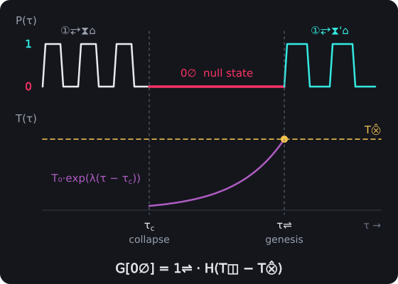
Collapse and Genesis. At the collapse time τ_c the pulse falls to the null state, P(τ_c) = 0. Boundary tension then grows as T₀ · exp(λ(τ − τ_c)) until it reaches the threshold T⨶ at τ⇌, where the step G[0∅] = 1⇌ · H(T◫ − T⨶) starts the child's pulse sequence at its own Tempo ①⥂⧗'⌂.
Genesis Transition Function G
G: {0∅} → {1⇌} [∅]
Where:
- G [∅] - genesis transition function
- 0∅ [∅] - null state representation
- → - mapping operator indicating transformation
- 1⇌ [∅] - genesis state representation
- [∅] - quantities without physical units, pure numerical ratios or mathematical constants
Dimensional analysis:
Where (from the book): G [∅], 0∅ [∅], 1⇌ [∅], [∅] [∅]
Read dimensionally: G: (0∅) → (1⇌)
[∅] : ([∅]) → ([∅]) = [∅] : [∅] → [∅] ✓ Valid PulseCore Verified ✓
➢ Discrete transition from null to active state, framing cosmic creation as computational state transformation.
Discrete Genesis Step Function
G[0∅] = 1⇌ · H(T◫ - T⨶) [∅]
Where:
- G[0∅] [∅] - genesis function applied to null state
- H [∅] - Heaviside step function ensuring discrete transition
- T◫ [𝕄·𝕃²·𝕋⁻²] - boundary tension energy
- T⨶ [𝕄·𝕃²·𝕋⁻²] - critical threshold energy
- [∅] - quantities without physical units, pure numerical ratios or mathematical constants
➢ Step function ensuring discrete genesis transition, addressing cosmic origin problems through threshold-activated computational reactivation mechanisms.
The Genesis Mechanism and Parameter Inheritance framework establishes the mathematical foundation for discrete cosmic creation through computational reactivation of Null Wells. The genesis condition defines precise energy thresholds for universe birth, while transition functions ensure discrete state changes from apparent physical suspension to active universe domains, reframing cosmic origins through threshold-activated reactivation mechanisms that transform accumulated boundary tension into new computational cycles with inherited physical parameters.
Parameter Inheritance and Constant Modification
Emergent Universes inherit modified parameters from Null Well characteristics. By studying the Parameter Inheritance and Constant Modification framework, we can understand how Null Well collapse events generate new universes with systematically modified fundamental constants, revealing the computational mechanisms underlying multiverse generation and the inheritance of physical parameters across cosmic cycles.
Inherited Planck Time
①⥂⧗'⌂ = ①⥂⧗⌂ × (M∅ / M_P)^(1/2) [𝕋]
Where:
- ①⥂⧗'⌂ [𝕋] - modified Pulse Tempo in emergent universe
- ①⥂⧗⌂ [𝕋] - original (parent) Pulse Tempo
- M∅ [𝕄] - Null Mass from computational collapse
- M_P [𝕄] - Planck mass
- ^(1/2) [∅] - square root exponent
- [∅] - quantities without physical units, pure numerical ratios or mathematical constants
Dimensional analysis:
Where (from the book): ^(1/2) [∅], [∅] [∅]
[𝕋]
[𝕋] × ([𝕄] ÷ [𝕄])^([∅] ÷ [∅]) = [𝕋] × ([𝕄] ÷ [𝕄])^([∅]) = [𝕋] × [∅]^([∅]) = [𝕋] × [∅] = [𝕋]
[𝕋] = [𝕋] ✓ Valid PulseCore Verified ✓
➢ Inherited temporal scaling from null mass, extending temporal foundations through mass-dependent modification of fundamental time scales.
Modified Constants
ℏ' = ℏ × (S_c / S_P)^α [𝕄·𝕃²·𝕋⁻¹]
Dimensional analysis:
[𝕄·𝕃²·𝕋⁻¹]
[𝕄·𝕃²·𝕋⁻¹] × ([∅] ÷ [∅])^([∅]) = [𝕄·𝕃²·𝕋⁻¹] × [∅]^([∅]) = [𝕄·𝕃²·𝕋⁻¹] × [∅] = [𝕄·𝕃²·𝕋⁻¹]
[𝕄·𝕃²·𝕋⁻¹] = [𝕄·𝕃²·𝕋⁻¹] ✓ Valid PulseCore Verified ✓
G' = G × (ρ∅ / ρ_P)^β [𝕄⁻¹·𝕃³·𝕋⁻²]
Dimensional analysis:
[𝕄⁻¹·𝕃³·𝕋⁻²]
[𝕄⁻¹·𝕃³·𝕋⁻²] × ([𝕄·𝕃⁻³] ÷ [𝕄·𝕃⁻³])^([∅]) = [𝕄⁻¹·𝕃³·𝕋⁻²] × [∅]^([∅]) = [𝕄⁻¹·𝕃³·𝕋⁻²] × [∅] = [𝕄⁻¹·𝕃³·𝕋⁻²]
[𝕄⁻¹·𝕃³·𝕋⁻²] = [𝕄⁻¹·𝕃³·𝕋⁻²] ✓ Valid PulseCore Verified ✓
𝒞→' = 𝒞→ × (E∅ / E_P)^γ [𝕃·𝕋⁻¹]
Where:
- ℏ' [𝕄·𝕃²·𝕋⁻¹] - modified reduced Planck constant
- ℏ [𝕄·𝕃²·𝕋⁻¹] - original reduced Planck constant
- S_c [∅] - critical entropy
- S_P [∅] - Planck entropy
- α [∅] - entropy scaling exponent
- G' [𝕄⁻¹·𝕃³·𝕋⁻²] - modified gravitational constant
- G [𝕄⁻¹·𝕃³·𝕋⁻²] - original gravitational constant
- ρ∅ [𝕄·𝕃⁻³] - null density
- ρ_P [𝕄·𝕃⁻³] - Planck density
- β [∅] - density scaling exponent
- 𝒞→' [𝕃·𝕋⁻¹] - modified speed of light
- 𝒞→ [𝕃·𝕋⁻¹] - original speed of light
- E∅ [𝕄·𝕃²·𝕋⁻²] - null energy
- E_P [𝕄·𝕃²·𝕋⁻²] - Planck energy
- γ [∅] - energy scaling exponent
- [∅] - quantities without physical units, pure numerical ratios or mathematical constants
Dimensional analysis:
Where (from the book): ℏ [𝕄·𝕃²·𝕋⁻¹], S_c [∅], α [∅], G' [𝕄⁻¹·𝕃³·𝕋⁻²], G [𝕄⁻¹·𝕃³·𝕋⁻²], ρ∅ [𝕄·𝕃⁻³], ρ_P [𝕄·𝕃⁻³], β [∅], E∅ [𝕄·𝕃²·𝕋⁻²], γ [∅], [∅] [∅]
[𝕃·𝕋⁻¹]
[𝕃·𝕋⁻¹] × ([𝕄·𝕃²·𝕋⁻²] ÷ [𝕄·𝕃²·𝕋⁻²])^([∅]) = [𝕃·𝕋⁻¹] × [∅]^([∅]) = [𝕃·𝕋⁻¹] × [∅] = [𝕃·𝕋⁻¹]
[𝕃·𝕋⁻¹] = [𝕃·𝕋⁻¹] ✓ Valid PulseCore Verified ✓
➢ Parameter inheritance through scaling relationships enabling multiverse with varying physics determined by Null Well collapse characteristics.
Dimensional Consistency Constraint
α²·β⁵ = γ·δ [∅]
Where:
- α [∅] - Planck time scale ratio ①⥂⧗'⌂/①⥂⧗⌂ (the ratios of Part 6.2, not the exponents α, β, γ of the laws above)
- β [∅] - light speed scale ratio 𝒞→'/𝒞→
- γ [∅] - gravitational constant scale ratio G'/G
- δ [∅] - Planck constant scale ratio ℏ'/ℏ
- [∅] - quantities without physical units, pure numerical ratios or mathematical constants
Dimensional analysis:
Where (from the book): α [∅], β [∅], γ [∅], δ [∅], [∅] [∅]
[∅] × [∅] = [∅]
[∅] × [∅] = [∅]
[∅] = [∅] ✓ Valid PulseCore Verified ✓
➢ It follows from ①⥂⧗⌂ = √(ℏG/𝒞→⁵): (①⥂⧗'⌂/①⥂⧗⌂)² = (ℏ'/ℏ)(G'/G)/(𝒞→'/𝒞→)⁵, so α²·β⁵ = γ·δ, the consistency rule of Part 6.2 that every inherited set of constants must keep.
Universe Classification by Genesis Parameters
Null Mass | M∅/M_P | Child's Tempo ①⥂⧗′⌂/①⥂⧗⌂ | Genesis Type | Universe Characteristics |
|---|---|---|---|---|
Super-Critical | 10⁶ | 10³ | Hyper-Genesis | Slow-pulsing and long-lived; every pulse carries 10³ times the bits |
Critical | 1 | 1 | Standard Genesis | Pulses at its parent's Local Pulse Tempo; normal evolution |
Failed | any | — | Failed Genesis | Seeds no child; its data returns to the Source without continuing back (Part 3.9) |
Where:
- M∅ [𝕄] - Null Mass from computational collapse
- M_P [𝕄] - Planck mass
- 10⁶ [∅] - super-critical mass ratio threshold
- 1 [∅] - critical mass ratio threshold
- ①⥂⧗′⌂/①⥂⧗⌂ [∅] - the child's Local Pulse Tempo relative to its parent's, (M∅/M_P)^½
- [∅] - quantities without physical units, pure numerical ratios or mathematical constants
Dimensional analysis: [𝕄]/[𝕄] = [∅] ✓ The universe classification ratios are dimensionally consistent as mass ratios.
➢ No Null Well forms below one Planck mass, so a mass ratio below 1 is not a universe class. A heavier well gives a slower child, ①⥂⧗′⌂ = ①⥂⧗⌂ · (M∅/M_P)^½ (Part 6.5): it carries more bits in every pulse and lives longer in its parent's time. Failure is not set by mass: a collapse that falls short of the data-energy threshold seeds no child whatever its mass (Part 3.9). A merger-compressed core is the exception to slower (Part 6.5): it can give a faster child, never faster than ℨ.
The Parameter Inheritance and Constant Modification framework demonstrates how Binary Pulse Theory enables multiverse generation through systematic modification of fundamental constants based on Null Well collapse characteristics, with inherited parameters following scaling relationships that maintain dimensional consistency while enabling universes with systematically different physics.
➢ Read with the Level and Lineage Clock (Part 2.8). A heavier well gives a slower child; in the clock as now written that is carried by level, the child's level growing with its well's mass (Level from Mass, Part 3.14) and its clock doubling with each level, ①⥂⧗⌂ = ℨ · 2^L · H. The square-root form here was the first reading of it and gives a different step between generations; the clock law is the one the game and the lineage reading use.
Universal Cyclical Evolution and Temporal Dynamics
Universe evolution follows predictable cyclical patterns:
Evolution Phases:
- Genesis Phase: Rapid expansion and structure formation
- Maturation Phase: Complex dynamics and entropy accumulation
- Senescence Phase: Energy dissipation and Pulse deceleration
- Collapse Phase: Return to null state and new genesis preparation
Penrose's conformal cyclic cosmology (Penrose, 2010) shares conceptual commonalities with cyclical evolution, where one Universe's end becomes the next's beginning.
Cycle Duration G
T⟳ = (2π/H') · ln(S⥣/S⥥) [𝕋]
Where:
- T⟳ [𝕋] - complete evolution cycle duration
- π [∅] - mathematical constant pi
- H' [𝕋⁻¹] - effective Hubble parameter in emergent Universe
- ln - natural logarithm function
- S⥣ [∅] - maximum entropy
- S⥥ [∅] - minimum entropy
- [∅] - quantities without physical units, pure numerical ratios or mathematical constants
Dimensional analysis:
Where (from the book): π [∅], S⥣ [∅], [∅] [∅]
[𝕋]
([∅] × [∅] ÷ [𝕋⁻¹]) × ln([∅] ÷ [∅]) = ([∅] ÷ [𝕋⁻¹]) × ln([∅] ÷ [∅]) = [𝕋] × ln([∅] ÷ [∅]) = [𝕋] × ln([∅]) = [𝕋] × [∅] = [𝕋]
[𝕋] = [𝕋] ✓ Valid PulseCore Verified ✓
➢ Complete evolution cycle duration enabling cosmic renewal through entropy-driven temporal scaling.
Entropy Evolution
S(τ) = S⥥ + (S⥣ - S⥥) · (1 - exp(-τ/τ_S)) [∅]
Where:
- S(τ) [∅] - entropy as function of proper time
- τ [𝕋] - proper time variable
- S⥥ [∅] - minimum entropy
- S⥣ [∅] - maximum entropy
- exp - exponential function
- τ_S [𝕋] - entropy evolution timescale
- [∅] - quantities without physical units, pure numerical ratios or mathematical constants
Dimensional analysis:
Where (from the book): τ [𝕋], [∅] [∅]
[∅]
[∅] + ([∅] - [∅]) × ([∅] - exp([𝕋] ÷ [𝕋])) = [∅] + [∅] × ([∅] - exp([𝕋] ÷ [𝕋])) = [∅] + [∅] × ([∅] - exp([∅])) = [∅] + [∅] × ([∅] - [∅]) = [∅] + [∅] × [∅] = [∅] + [∅] = [∅]
[∅] = [∅] ✓ Valid PulseCore Verified ✓
➢ Connection to intergenerational parameter inheritance enabling cosmic evolution through systematic entropy accumulation and cyclical renewal mechanisms.
The Universal Cyclical Evolution and Temporal Dynamics framework demonstrates how Binary Pulse Theory governs cosmic evolution through predictable four-phase cycles, with cycle duration determined by entropy ratios and Hubble scaling, while entropy evolution follows exponential temporal dynamics that enable systematic parameter inheritance across cosmic generations.
Comparison with Classical Cosmological Models
BPT Null Well Genesis versus Standard Big Bang
Aspect | Big Bang Model | BPT Null Well Model |
|---|---|---|
Initial State | Undefined singularity | Well-defined null state |
Genesis Mechanism | Explosive expansion | Computational reactivation |
Information Fate | Lost at singularity | Preserved in boundary encoding I◫ |
Causality Origin | Light cone emergence | Recursive Pulse propagation |
Time Genesis | Continuous from t=0 | Discrete at τ=τ⇌ |
Where:
- P(τ_c) [∅] - pulse state at collapse time, well-defined null state
- τ_c [𝕋] - collapse time
- G[0∅] [∅] - genesis function applied to null state
- 0∅ [∅] - null state representation
- 1⇌ [∅] - genesis state representation
- I◫ [1ᵇ] - surface information content preserved in boundary
- τ⇌ [𝕋] - genesis activation time
- t [𝕋] - continuous time variable in Big Bang model
- [∅] - quantities without physical units, pure numerical ratios or mathematical constants
6.7 Testable Predictions
The predictions this part shares with Chapter 2 are listed in Part 2.7.
If confirmed, these predictions would support collapse as creative necessity, showing that:
- Cosmic collapse preserves rather than destroys information