Chapter 9 · Section 1
Dark Matter — Computational Resolution Failures
Dark Matter as Unresolved Computation
The Universe's most perplexing puzzle — requiring five times more gravitational mass than visible matter provides — finds a computational reading in Binary Pulse Theory's identification of dark matter as Unresolved Computational Nodes. Rather than exotic particles existing beyond the Standard Model, these incomplete Pulse resolution events within the discretized binary substrate generate gravitational effects without electromagnetic interaction. Part 3.13 names them: the data that never resolved into matter at the Physical Nova is Data Matter, carrying mass by the Data–Matter Equivalence and no charge to touch light with, laid on the scaffold before ordinary matter falls into it.
This reading recasts dark matter from the "Missing Mass Problem" into a predictable computational phenomenon. Building upon Pulse Rhythm relationships ①⥂⧖♁ = ①⥂⧗♁/2 [𝕋] (the Rhythm is the one-way traverse, half of the full Local Pulse Tempo ①⥂⧗♁, the Planck time, t_P ≈ 5.39 × 10⁻⁴⁴ s), dark matter emerges naturally from Partial State Transitions that influence spacetime curvature while remaining electromagnetically invisible.
Bertone, Hooper, and Silk's comprehensive analysis (Bertone et al., 2005)¹ established robust evidence for dark matter phenomena across multiple observational scales. Clowe and colleagues' direct empirical proof (Clowe et al., 2006)² demonstrated the necessity of non-baryonic mass components through gravitational lensing observations. Recent Planck Collaboration measurements (Planck Collaboration, 2020)³ provide precise quantification of the dark matter fraction, which Binary Pulse Theory reads as a sign that the Universe's large-scale structure reflects substrate-level computational dynamics.
Unlike conventional matter arising from fully resolved Prime Pulse Bifurcation ∅ → (0 ↔ 1) transitions generating quantized mass-energy and electromagnetic interactions, Unresolved Computational Nodes represent incomplete recursive processes that manifest as gravitational mass through Information Conservation I⊚ = I▱ + Iℜ principles, addressing Weinberg's cosmological constant problem (Weinberg, 1989)⁴ through computational rather than fine-tuning explanations.
Mathematical Framework for Computational Dark Matter
Dark matter emerges not as exotic new particles but as a computational byproduct: unresolved nodes within the substrate where resolution fails. At the Zinf-Limit, these failures manifest as hidden densities, gravitationally active yet electromagnetically silent, arising directly from Information Conservation constraints. Dark matter density emerges from Computational Substrate Resolution Failures (G) following Information Conservation principles. This builds upon Zwicky's foundational observations (Zwicky, 1933)⁵ of discrepancies requiring additional gravitational mass beyond visible matter.
Resolution Function G
R(x,t) = Σₙ P_n(x,t) × H(Tₙ - T⨶) [∅]
Where:
- R(x,t) [∅] - resolution function
- Σ [∅] - summation operator
- n [∅] - pulse state index
- P_n(x,t) [∅] - nth pulse state amplitude
- x [𝕃] - spatial position vector
- t [𝕋] - time variable
- H [∅] - Heaviside step function
- Tₙ [𝕋] - threshold time for nth pulse resolution
- T⨶ [𝕋] - critical resolution time threshold
Dimensional analysis:
Where (from the book): Σ [∅], n [∅], x [𝕃], t [𝕋], H [∅], T⨶ [𝕋]
Read dimensionally: R(x,t) = P_n(x,t) × H(Tₙ - T⨶)
[∅]
[∅] × [∅]([𝕋] - [𝕋]) = [∅] × [∅]([𝕋]) = [∅] × [∅] = [∅]
[∅] = [∅] ✓ Valid PulseCore Verified ✓
➢ The Resolution Function quantifies computational completeness, where incomplete resolution creates unresolved nodes contributing to dark matter effects through substrate coupling mechanisms, demonstrating how threshold-dependent summation establishes completeness assessment that characterizes unresolved node formation and dark matter contributions through incomplete computational resolution in substrate architectures.
The Pulse Resolution Rate G
α(x,t) = ⟨R(x,t)⟩/⟨P⊚(x,t)⟩ [∅]
Where:
- α(x,t) [∅] - pulse resolution rate
- ⟨⟩ [∅] - ensemble average operator
- R(x,t) [∅] - resolved activity
- P⊚(x,t) [∅] - total pulse state amplitude
- x [𝕃] - spatial position vector
- t [𝕋] - time variable
Dimensional analysis:
Where (from the book): x [𝕃], t [𝕋]
Read dimensionally: α(x,t) = (R(x,t))/(P⊚(x,t))
[∅]
([∅]) ÷ ([∅]) = [∅] ÷ [∅] = [∅]
[∅] = [∅] ✓ Valid PulseCore Verified ✓
➢ The Pulse Resolution Rate quantifies computational processing effectiveness through resolution efficiency measurement, demonstrating how the ratio of resolved to total pulse activity establishes performance assessment that characterizes computational processing effectiveness and resolution performance in substrate architectures.
Total Pulse Amplitude
P⊚(x,t) = Σₙ |P_n(x,t)|² [∅]
Where:
- P⊚(x,t) [∅] - total pulse amplitude across states
- Σ [∅] - summation operator
- n [∅] - pulse state index
- P_n(x,t) [∅] - individual pulse state amplitudes
- x [𝕃] - spatial position vector
- t [𝕋] - time variable
Dimensional analysis:
Where (from the book): Σ [∅], n [∅], x [𝕃], t [𝕋]
Read dimensionally: P⊚(x,t) = (abs(P_n(x,t)))²
[∅]
(abs([∅]))² = [∅]² = [∅]
[∅] = [∅] ✓ Valid PulseCore Verified ✓
➢ Pulse Resolution Rate quantifies the fraction of resolved activity relative to the total, with α = 1 indicating complete resolution, demonstrating how squared amplitude summation establishes total pulse energy that characterizes the denominator for resolution efficiency assessment where complete resolution represents optimal computational processing in substrate architectures.
Unresolved Node Density quantifies how incomplete Pulse resolution creates density concentrations affecting spacetime geometry without electromagnetic visibility.
Unresolved Node Density G
ρ⬚(x,t) = ρ▱ × (1 - α(x,t))² [𝕄·𝕃⁻³]
Where:
- ρ⬚(x,t) [𝕄·𝕃⁻³] - unresolved node density
- ρ▱ [𝕄·𝕃⁻³] - base computational substrate density
- 1 [∅] - unity constant
- α(x,t) [∅] - pulse resolution rate
- x [𝕃] - spatial position vector
- t [𝕋] - time variable
Dimensional analysis:
Where (from the book): 1 [∅], ρ⬚(x,t) [𝕄·𝕃⁻³], ρ▱ [𝕄·𝕃⁻³], x [𝕃], t [𝕋]
[𝕄·𝕃⁻³]
[𝕄·𝕃⁻³] × ([∅] - [∅])² = [𝕄·𝕃⁻³] × [∅]² = [𝕄·𝕃⁻³] × [∅] = [𝕄·𝕃⁻³]
[𝕄·𝕃⁻³] = [𝕄·𝕃⁻³] ✓ Valid PulseCore Verified ✓
➢ Regions with lower resolution rates exhibit higher unresolved node density, creating gravitational effects without electromagnetic coupling — offering a computational account of dark matter, demonstrating how computational incompleteness establishes dark matter density that characterizes gravitational effects without electromagnetic interaction through unresolved computational processes in substrate architectures.
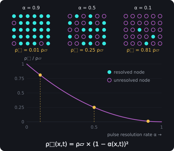
Unresolved Node Density. Where a region resolves a fraction α of its pulse activity, the rest stays as unresolved nodes: ρ⬚ = ρ▱ × (1 − α)². Full resolution leaves no unresolved density; at α = 0.5 a quarter of the substrate density remains, and at α = 0.1 most of it.
Dark Matter Density Relation G
ρ_DM(x,t) = n⬚(x,t) × ρ≡ × G⧱(∇²α) [𝕄·𝕃⁻³]
Where:
- ρ_DM(x,t) [𝕄·𝕃⁻³] - dark matter density
- n⬚(x,t) [𝕃⁻³] - number density of unresolved nodes
- ρ≡ [𝕄] - effective gravitational mass per unresolved node
- G⧱(∇²α) [∅] - gravitational coupling function
- ∇² [𝕃⁻²] - Laplacian operator
- α [∅] - pulse resolution rate
- x [𝕃] - spatial position vector
- t [𝕋] - time variable
Dimensional analysis:
Where (from the book): ρ_DM(x,t) [𝕄·𝕃⁻³], n⬚(x,t) [𝕃⁻³], G⧱(∇²α) [∅], α [∅], x [𝕃], t [𝕋]
[𝕄·𝕃⁻³]
[𝕃⁻³] × [𝕄] × [∅] = [𝕄·𝕃⁻³] × [∅] = [𝕄·𝕃⁻³]
[𝕄·𝕃⁻³] = [𝕄·𝕃⁻³] ✓ Valid PulseCore Verified ✓
➢ Gravitational coupling depends on resolution field curvature, connecting computational incompleteness to spacetime geometry modifications through substrate architecture, demonstrating how resolution field curvature establishes gravitational coupling that characterizes the connection between computational incompleteness and spacetime geometry through unresolved node density effects in substrate architectures.
Thus, what astronomers detect as missing mass is reinterpreted as computational incompleteness—regions where Pulse resolution remains partial, leaving residual gravitational imprint. In this light, dark matter is revealed as the shadow of unresolved computation, a structural consequence of the substrate’s finite resolution rather than an independent form of matter.
Substrate Computational Architecture
The substrate is not a uniform continuum but a binary lattice, discretized at the Planck scale and organized into a hierarchical architecture anchored by Pulse timing. From fully resolved Planck states to partially resolved galactic structures, resolution efficiency cascades through nested levels, shaping the very distribution of visible and invisible matter.
Binary substrate exhibits hierarchical resolution structure anchored to fundamental Pulse timing, following principles demonstrated in Ashtekar and Lewandowski's background-independent quantum gravity (Ashtekar & Lewandowski, 2004)⁶. The Substrate Lattice operates with spacing a = lₚ = (ℏG/𝒞→³)^(1/2) [𝕃], containing N_nodes = (L/lₚ)³ [∅] computational nodes for volume L³ [𝕃³].
Resolution Hierarchy spans multiple scales:
- Tier 0: Planck-scale binary states (fully resolved)
- Tier 1: Atomic-scale structures (nearly fully resolved)
- Tier 2: Molecular complexes (mostly resolved)
- Tier 3: Macroscopic objects (mixed resolution)
- Tier 4: Galactic scales (partially resolved: unresolved components — dark matter signature)
The Resolution Transfer Function governs how resolution efficiency decreases with scale, connecting to Lloyd's computational capacity research (Lloyd, 2002)⁷.
Resolution Transfer Function G
α_{n+1} = αₙ × T⊶(Lₙ/L_{n+1}) [∅]
Where:
- α_{n+1} [∅] - resolution efficiency at tier n+1
- αₙ [∅] - resolution efficiency at tier n
- T⊶ [∅] - transfer function between scales, at most 1, so resolution efficiency never rises from one tier to the next
- Lₙ [𝕃] - characteristic length at tier n
- L_{n+1} [𝕃] - characteristic length at tier n+1
- n [∅] - scale tier index
Dimensional analysis:
Where (from the book): αₙ [∅], T⊶ [∅], Lₙ [𝕃], L_{n+1} [𝕃], n [∅]
[∅]
[∅] × [∅]([𝕃] ÷ [𝕃]) = [∅] × [∅]([∅]) = [∅] × [∅] = [∅]
[∅] = [∅] ✓ Valid PulseCore Verified ✓
➢ Resolution efficiency decreases systematically with increasing scale, creating predictable dark matter signatures at galactic and cosmological levels, demonstrating how scale-dependent transfer mechanisms establish hierarchical dark matter distribution that characterizes systematic resolution degradation across cosmic scales through transfer function relationships in substrate architectures.
In this view, cosmic structure reflects the substrate’s resolution hierarchy itself, with dark matter emerging as the predictable shadow of scale-dependent inefficiency. What appears astrophysically as hidden mass is, at root, a computational trace of how resolution is transferred and degraded across levels of the binary lattice.
Dark Energy as Recursive Expansion Pressure
Dark energy emerges from the Global Recursion Tension Imbalance of uncollapsed states, which acts like the negative-pressure terms in the Einstein field equations. Weinberg's cosmological constant problem (Weinberg, 1989)⁴ would then find a computational resolution rather than a fine-tuning explanation. The uncollapsed states are the Data Matter, and the space they return to is the emptied Pulsecore, the Null Vacuum: its outward push is the Vacuum Pressure of Part 3.13, supplied by the returning data, which is why its equation of state evolves.
Global Recursion Tension Imbalance G
T◁⦰(t) = ∫ T⌂(x,t) × (1 - α(x,t)) d³x [N·m]
Where:
- T◁⦰(t) [𝕄·𝕃²·𝕋⁻²] - global recursion tension imbalance
- ∫ [∅] - integration operator
- T⌂(x,t) [𝕄·𝕃⁻¹·𝕋⁻²] - local tension density
- x [𝕃] - spatial position vector
- 1 [∅] - unity constant
- α(x,t) [∅] - local resolution efficiency
- d³x [𝕃³] - volume element
- t [𝕋] - time variable
Dimensional analysis:
Where (from the book): 1 [∅], T⌂(x,t) [𝕄·𝕃⁻¹·𝕋⁻²], x [𝕃], t [𝕋]
Read dimensionally: T◁⦰(t) = T⌂(x,t) × (1 - α(x,t)) × d³x
[𝕄·𝕃²·𝕋⁻²]
[𝕄·𝕃⁻¹·𝕋⁻²] × ([∅] - [∅]) × [𝕃³] = [𝕄·𝕃⁻¹·𝕋⁻²] × [∅] × [𝕃³] = [𝕄·𝕃⁻¹·𝕋⁻²] × [𝕃³] = [𝕄·𝕃²·𝕋⁻²]
[𝕄·𝕃²·𝕋⁻²] = [𝕄·𝕃²·𝕋⁻²] ✓ Valid PulseCore Verified ✓
➢ Unresolved recursive processes create tension manifesting as cosmic expansion pressure through computational dynamics rather than mysterious "dark energy" fields, demonstrating how computational incompleteness establishes expansion pressure that characterizes cosmic acceleration through unresolved recursive tension rather than dark energy mechanisms in substrate architectures.
In this light, dark energy is not a mysterious external field but the emergent pressure of unresolved recursion, with expansion driven by the tension imbalance of uncollapsed states. What general relativity encodes as a cosmological constant is, in Binary Pulse Theory, the computational signature of incompleteness itself.
Dark Matter From Other Domains — Matter We Are Not Tuned To
Gravity is data density on the grid (Part 1.11), and every Harmonic Domain shares the same pixels (Part 1.9), so data held at any level where we are adds to the curvature we feel. Light is not shared. It is a pattern at one domain’s own scale and frequency, and to see it is to be tuned to it, the same tuning an interdomain craft must make (Part 9.5). Whatever other domains hold here is felt and not seen: dark matter is, in part, matter we are not tuned to. Physics has met the same shape before, a hidden sector that shares only gravity with ours: the shadow matter of superstring theories (Kolb, Seckel & Turner, 1985) and the brane worlds in which gravity alone reaches the space around them (Randall & Sundrum, 1999).
How much of it there can be is already fixed. Our own Data Matter, counted at the Physical Nova, gives a dark-to-ordinary ratio of (1 − 2^(−D)) × 144/25 = 27/5 = 5.40 for four actual dimensions (Part 3.13), against the measured 5.36 ± 0.06 (Planck Collaboration, 2020). The count leaves very little room.
Interdomain Dark Share G
ε⇄ = 1 − (1 − 2^(−D)) × (144 / 25) × ρ_b / ρ◍ [∅]
Dimensional analysis:
Where (from the book): ε⇄ [∅], D [∅], ρ_b [𝕄·𝕃⁻³]
[∅]
[∅] - ([∅] - [∅]^([∅])) × ([∅] ÷ [∅]) × [𝕄·𝕃⁻³] ÷ [𝕄·𝕃⁻³] = [∅] - ([∅] - [∅]^([∅])) × ([∅] ÷ [∅]) × [𝕄·𝕃⁻³] ÷ [𝕄·𝕃⁻³] = [∅] - ([∅] - [∅]) × ([∅] ÷ [∅]) × [𝕄·𝕃⁻³] ÷ [𝕄·𝕃⁻³] = [∅] - [∅] × ([∅] ÷ [∅]) × [𝕄·𝕃⁻³] ÷ [𝕄·𝕃⁻³] = [∅] - [∅] × [∅] × [𝕄·𝕃⁻³] ÷ [𝕄·𝕃⁻³] = [∅] - [∅] × [𝕄·𝕃⁻³] ÷ [𝕄·𝕃⁻³] = [∅] - [𝕄·𝕃⁻³] ÷ [𝕄·𝕃⁻³] = [∅] - [∅] = [∅]
[∅] = [∅] ✓ Valid PulseCore Verified ✓
The share of the dark matter that our own Data Matter does not count
Where:
- ε⇄ [∅] — the share of the measured dark matter left over once our own Data Matter is counted: the most other domains can hold where we are
- (1 − 2^(−D)) × 144/25 [∅] — our Data Matter per unit of ordinary matter, from the counts (Part 3.13)
- ρ_b, ρ◍ [𝕄·𝕃⁻³] — the measured densities of ordinary and dark matter
➢ Our sky gives ε⇄ = 1 − 5.40 / 5.36 = −0.007 ± 0.011: no share from other domains is needed, and at two standard deviations they can hold at most about 1.5 % of the dark matter. Other domains are not where dark matter comes from; they can add at most a trace, and the count of our own Data Matter is the test passed. The bound reaches further than dark matter. A craft that can tune to a domain from here shows that the domain’s data is here, and that data’s gravity reaches us: interdomain travel and interdomain gravity are one coupling, and the measured ratio bounds how much every other domain holds where we are.
A trace would show in two ways. A part spread evenly acts only on the expansion, not on the clumping, so it would appear as a small difference between the matter measured from the expansion and the matter measured from clustering; measurements of clustering already sit slightly below the value the expansion leads one to expect (Heymans et al., 2021), the place a trace would be looked for, not evidence of one. A part that gathers would be pulled into our own wells and follow our matter, a little more mass in every halo than our Data Matter accounts for.
9.1 Testable Predictions
- Resolution-dependent Dark Matter Profiles exhibiting characteristic deviations from NFW Profiles in high-resolution regions where computational completion approaches unity, detectable through gravitational lensing analysis with mass profile reconstruction precision better than 5% at sub-kpc scales.
- Dark Energy Equation of State Evolution: Showing time-dependent deviations from cosmological constant behavior through Recursive Tension Dynamics, measurable in supernova distance-redshift relationships with w(z) parameter evolution tracking over cosmic time.
- Gravitational Lensing Modifications: Producing Resolution Gradient Signatures detectable in strong lensing systems with angular resolution better than 0.1 arcseconds, revealing systematic distortions in Einstein ring geometries at computational boundaries.
- Cosmic Microwave Background Anisotropies: Modified by resolution fluctuations through enhanced transfer functions at specific angular scales around ℓ ≈ 1000, observable as excess power spectral density deviations from standard ΛCDM predictions.
- Galaxy Cluster Dynamics: Showing Dark Matter Heating Effects in high-resolution central regions approaching complete computational resolution, measurable through velocity dispersion profiles exhibiting temperature increases toward cluster cores.
- Hubble Tension Resolution: Through time-dependent dark energy evolution connecting early and late Universe expansion rates, quantifiable as H₀ convergence within 1σ uncertainty when recursive tension effects are incorporated into distance ladder measurements.
- Interdomain Dark Share: as the measured dark-to-ordinary ratio tightens, ε⇄ = 1 − 5.40 × ρ_b / ρ◍ must stay at or near zero. A ratio settled clearly above 5.40 would measure a share held by other domains; one settled clearly below would fail the count of Part 3.13.
These predictions offer a testable framework for understanding dark matter and dark energy as computational phenomena rather than exotic physics. Binary Pulse Theory's identification of dark matter as unresolved computational nodes offers an account of one of physics' greatest open questions while opening new frontiers in computational cosmology.