Chapter 9 · Section 2
Temporal Resolution — Density-Dependent Time
Time Has Variable Resolution
What determines the fundamental temporal resolution of emergent Universes — the shortest meaningful duration between distinguishable causal states? Binary Pulse Theory proposes spacetime itself as a discrete computational substrate operating through irreducible binary transitions, where Prime Pulse Bifurcation ∅ → (0 ↔ 1) defines the minimal causal increment governing all physical processes.
This insight proposes that time resolution varies with computational density, inverting the usual picture of temporal fundamentals. Instead of Planck time being a universal constant, it emerges from Density-Dependent Emergence mechanisms that connect collapse conditions to computational capacity.
Ashtekar and Lewandowski's background-independent quantum gravity (Ashtekar & Lewandowski, 2004)⁶ demonstrates how geometry emerges from fundamental quantum states rather than existing as fixed spacetime stage. Building upon Pulse Rhythm Definition ①⥂⧖⌂ = ①⥂⧗⌂/2 [𝕋] (one way is half of a full pulse; the Local Pulse Tempo ①⥂⧗⌂ = t_P), discretization manifests at quantum scales through density-encoded mechanisms governing Universe formation.
Lloyd's computational capacity research (Lloyd, 2002)⁷ and Wheeler's "It from Bit" concept (Wheeler, 1989)¹ provide frameworks for understanding how Collapse Density ρ⦰ modulates emergent Planck time through gravitational scaling laws. The resulting temporal resolution determines information processing capacity and complexity potential of newly formed cosmic domains.
Information Conservation I⊚ = I▱ + Iℜ connects directly to Temporal Grain Size supporting recursive processing. Emergent Universes inherit computational substrate characteristics from parent Null Well collapse density, creating mathematical relationships between collapse conditions and temporal resolution capabilities through mechanisms demonstrated in Smolin's cosmological natural selection (Smolin, 1997)⁸ and Penrose's conformal cyclic cosmology (Penrose, 2010)⁹.
Mathematical Foundation of Computational Time
The mathematical foundation of computational time begins at the Planck scale, where physical constants converge to define the minimal tick of reality. Binary Pulse Theory reframes this not as a fixed boundary, but as the baseline of resolution from which deeper computational timing emerges. Planck scale operates as Binary Resolution Baseline through the established Pulse Duration Framework (G). Standard Planck time emerges from fundamental constants.
Standard Planck Time
t_P = (ℏG/c⁵)^(1/2) ≈ 5.391 × 10^(-44) × s [𝕋]
Where:
- ℏ [𝕄·𝕃²·𝕋⁻¹] - reduced Planck constant = 1.055 × 10^(-34) J·s
- G [m³/(kg·s²)] - gravitational constant = 6.674 × 10^(-11) m³/(kg·s²)
- c [𝕃·𝕋⁻¹] - speed of light = 2.998 × 10^8 m/s
➢ Planck time represents the fundamental temporal quantum below which spacetime geometry becomes undefined — but BPT proposes that this emerges from deeper computational processes.
Density-Encoded Emergence Relation modulates temporal resolution based on collapse conditions:
Density-Encoded Emergence Relation G
①⥂⧗'⌂ = (ℏ'G'/𝒞→'⁵)^(1/2) = ①⥂⧗⌂ × f(ρ⦰) [𝕋]
Where:
- ①⥂⧗'⌂ [𝕋] - modified Local Pulse Tempo (the emergent Universe's Planck time)
- ℏ' [𝕄·𝕃²·𝕋⁻¹] - modified reduced Planck constant
- G' [𝕄⁻¹·𝕃³·𝕋⁻²] - modified gravitational constant
- 𝒞→' [𝕃·𝕋⁻¹] - modified speed of light
- f(ρ⦰) [∅] - density scaling function ((ρ⨶/ρ⦰)^(1/2))
- ①⥂⧗⌂ [𝕋] - Local Pulse Tempo (standard Planck time)
- ρ⦰ [𝕄·𝕃⁻³] - density at Universe formation
- ρ⨶ [𝕄·𝕃⁻³] - critical density threshold: the parent's Planck density ρ_P = 𝒞→⁵/(ℏG²) ≈ 5.16 × 10⁹⁶ kg/m³, which a single collapse does not exceed
- 1/2 [∅] - scaling exponent
➢ Collapse density sets each emergent Universe's temporal resolution. A single collapse stays below its parent's Planck density, so most children receive a coarser resolution and pulse more slowly than their parent; only a core compressed past that density, through a merger or the merger-built core of a supermassive well, receives a finer resolution and a faster pulse, and none passes the Zinf limit ℨ — explaining why different universes exhibit different temporal characteristics, demonstrating how density-dependent temporal scaling establishes sophisticated processing capability that characterizes Universe formation dynamics through computational resolution enhancement in substrate architectures.
Time is not a fixed backdrop but a recursive product of the substrate itself, tightening its resolution under higher collapse densities. Within Binary Pulse Theory, Planck time serves only as the baseline: each universe’s temporal granularity is set by the density of the collapse that formed it, and stays fixed within that universe.
Recursive Inheritance and Computational Scaling
Recursive Inheritance and Computational Scaling describes how temporal resolution is not fixed at a single baseline but inherited and reshaped across collapse densities and successive universes. By tying Planck-scale intervals to density-dependent modulation, Binary Pulse Theory reframes computational capacity as a dynamic property that flexes with the conditions of formation.
Temporal Resolution Ratio R⧗ = ①⥂⧗'⌂/①⥂⧗⌂ = f(ρ⦰) [∅] determines computational capacity scaling. Information Processing Capacity scales as I◉ ∝ 1/①⥂⧖' ∝ 1/f(ρ⦰) [𝕋⁻¹], creating distinct computational regimes.
Collapse Density Regimes G
Density Range | Temporal Resolution | Computational Implications |
|---|---|---|
ρ⦰ ≫ ρ⨶ | ①⥂⧖' ≪ ①⥂⧖ | Ultra-high frequency processing (merger-compressed cores only) |
ρ⦰ ≈ ρ⨶ | ①⥂⧖' ≈ ①⥂⧖ | Similar computational capacity |
ρ⦰ ≪ ρ⨶ | ①⥂⧖' ≫ ①⥂⧖ | Coarse-grained temporal evolution |
Where:
- ρ⦰ [𝕄·𝕃⁻³] - density at Universe formation
- ρ⨶ [𝕄·𝕃⁻³] - critical density threshold
- ①⥂⧖' [𝕋] - modified Pulse Rhythm
- ①⥂⧖ [𝕋] - standard Pulse Rhythm
➢ Collapse Density Regimes establish density-dependent computational capacity scaling through temporal resolution variation, demonstrating how different collapse densities create distinct processing characteristics that characterize Universe formation outcomes ranging from ultra-high frequency processing to coarse-grained temporal evolution in substrate architectures.
Multi-Generational Scaling
①⥂⧗⌂⁽ⁿ⁾ = ①⥂⧗⌂⁽⁰⁾ × ∏_{i=1}^n f(ρᵢ) [𝕋]
Where:
- ①⥂⧗⌂⁽ⁿ⁾ [𝕋] - Planck time in nth generation Universe
- ①⥂⧗⌂⁽⁰⁾ [𝕋] - initial Planck time (zeroth generation)
- ∏ [∅] - product operator
- i [∅] - generation index
- 1 [∅] - product lower limit
- n [∅] - generation number
- f(ρ_i) [∅] - density scaling function at generation i
- ρᵢ [𝕄·𝕃⁻³] - collapse density at generation i
Dimensional analysis:
Where (from the book): 1 [∅], ①⥂⧗⌂⁽ⁿ⁾ [𝕋], ①⥂⧗⌂⁽⁰⁾ [𝕋], i [∅], n [∅], f(ρᵢ) [∅]
Read dimensionally: ①⥂⧗⌂ = ①⥂⧗⌂ × prod(f(ρᵢ))
[𝕋]
[𝕋] × prod([∅]) = [𝕋] × [∅] = [𝕋]
[𝕋] = [𝕋] ✓ Valid PulseCore Verified ✓
➢ Temporal resolution inheritance across cosmic generations creates computational genealogy where processing capacity evolves systematically, demonstrating how cumulative density scaling establishes generation-dependent processing evolution that characterizes computational genealogy through systematic capacity development across cosmic generations in substrate architectures.
This framework connects to Polchinski's string theory (Polchinski, 1998) and Steinhardt and Turok's endless Universe model (Steinhardt & Turok, 2007), which offer settings in which Recursive State Evolution could operate across cosmic generations through density-dependent temporal architecture.
In this view, universes form a computational genealogy: each generation inherits temporal resolution from its predecessors yet modifies it through its own collapse density. What emerges is not a static timeline but a recursive lineage of processing architectures, scaling from ultra-fast substrates to coarse-grained evolutions — a framework that situates cosmic history itself as a chain of computational inheritances.
Null Well Collapse Integration
Null Well Collapse Integration formalizes the conditions under which a universe either stabilizes into coherent emergence or collapses into failure. By linking collapse density to threshold requirements, Binary Pulse Theory reframes the very act of dimensional birth as a computational selection process, where only certain densities yield viable substrates. The Threshold Density Relation determines emergence success.
Threshold Density Relation G
ρ⇗⨶ = (𝒞→⁵/(ℏG²)) × (①⥂⧗⌂/t✱)² [𝕄·𝕃⁻³]
Where:
- ρ⇗⨶ [𝕄·𝕃⁻³] - minimum density for stable emergence
- 𝒞→ [𝕃·𝕋⁻¹] - speed of light
- ℏ [𝕄·𝕃²·𝕋⁻¹] - reduced Planck constant
- G [𝕄⁻¹·𝕃³·𝕋⁻²] - gravitational constant
- t✱ [𝕋] - desired temporal resolution, the child's target Tempo
- ①⥂⧗⌂ [𝕋] - Local Pulse Tempo (standard Planck time)
Dimensional analysis:
Where (from the book): ℏ [𝕄·𝕃²·𝕋⁻¹], G [𝕄⁻¹·𝕃³·𝕋⁻²], t✱ [𝕋]
Read dimensionally: ρ⇗⨶ = (𝒞→⁵/(ℏ × G²)) × (①⥂⧗⌂/t✱)²
[𝕄·𝕃⁻³]
([𝕃⁵·𝕋⁻⁵] ÷ ([𝕄·𝕃²·𝕋⁻¹] × [𝕄⁻²·𝕃⁶·𝕋⁻⁴])) × ([𝕋] ÷ [𝕋])² = ([𝕃⁵·𝕋⁻⁵] ÷ [𝕄⁻¹·𝕃⁸·𝕋⁻⁵]) × ([𝕋] ÷ [𝕋])² = [𝕄·𝕃⁻³] × ([𝕋] ÷ [𝕋])² = [𝕄·𝕃⁻³] × [∅]² = [𝕄·𝕃⁻³] × [∅] = [𝕄·𝕃⁻³]
[𝕄·𝕃⁻³] = [𝕄·𝕃⁻³] ✓ Valid PulseCore Verified ✓
➢ The relation is the Density-Encoded Emergence Relation solved for density: ①⥂⧗'⌂ = ①⥂⧗♁ × (ρ⨶/ρ⦰)^(1/2) with ρ⨶ the Planck density 𝒞→⁵/(ℏG²) gives ρ⦰ = ρ⨶ × (①⥂⧗♁/t✱)². Each halving of the target Tempo takes four times the collapse density. At t✱ = ①⥂⧗♁ the threshold is the parent's Planck density, ≈ 5.16 × 10⁹⁶ kg/m³; any finer target lies beyond a single collapse and is reached only by a merger-compressed core; and the Zinf floor t✱ ≥ ℨ caps it, for our universe as parent, at ρ_P × s² ≈ 2.87 × 10²²¹ kg/m³, the Zinf density of Chapter 1. Higher target resolution therefore requires quadratically higher collapse densities, creating a natural selection mechanism for computational sophistication, demonstrating how density-dependent emergence thresholds establish computational evolution requirements that characterize natural selection for sophisticated processing through quadratic density scaling in substrate architectures.
Dimensional Emergence Conditions G
- Subcritical Density: ρ⦰ < ρ⇗⨶ → Failed emergence
- Critical Density: ρ⦰ = ρ⇗⨶ → Marginal emergence
- Supercritical Density: ρ⦰ > ρ⇗⨶ → Stable emergence with enhanced resolution
Where:
- ρ⦰ [𝕄·𝕃⁻³] - density at Universe formation
- ρ⇗⨶ [𝕄·𝕃⁻³] - minimum density for stable emergence
Dimensional analysis: [𝕄·𝕃⁻³] compared to [𝕄·𝕃⁻³] ✓ The Dimensional Emergence Conditions are dimensionally consistent for density threshold comparison.
➢ Dimensional Emergence Conditions establish density-dependent emergence outcomes through threshold comparison, demonstrating how density relative to critical thresholds determines Universe formation success that characterizes emergence criteria ranging from failed formation to stable emergence with enhanced computational resolution in substrate architectures.
These conditions can be compared with Ashtekar and Singh's loop quantum cosmology findings (Ashtekar & Singh, 2011) and with Barrow and Tipler's anthropic cosmological principle (Barrow & Tipler, 1986).
What emerges is a natural sieve at the foundation of reality: subcritical densities dissolve into failure, critical densities linger on the edge of instability, and only supercritical densities crystallize into coherent universes. In this framework, collapse itself becomes the cosmic filter — the recursive gate through which existence passes, ensuring that computational sophistication is reserved for those wells that achieve stable emergence.
Observational Signatures and Cosmic Structure
Variations in primordial density fluctuations produce testable signatures through multiple channels. Temperature Anisotropies follow δT/T ∝ f(ρ⦰) [∅] variations, while Polarization Patterns experience modification by Temporal Resolution Gradients. Spectral Distortions reflect different computational substrate properties across cosmic regions.
Large-Scale Structure Correlations manifest through subtle anisotropies in galaxy distribution patterns, Resolution Gradient Effects connecting to dark matter signatures, and coherent velocity flows indicating inherited collapse characteristics, in a discrete picture that draws on Sorkin's causal set theory (Sorkin, 2007).
Fundamental Constant Variations emerge through temporal resolution dependencies.
Modified Fine Structure Constant
α' = α × (①⥂⧗⌂/①⥂⧗'⌂)² = α/f(ρ⦰)² [∅]
Dimensional analysis:
[∅]
[∅] × ([𝕋] ÷ [𝕋])² = [∅] × [∅]² = [∅] × [∅] = [∅]
[∅] ÷ [∅] = [∅]
[∅] = [∅] = [∅] ✓ Valid PulseCore Verified ✓
The square follows from α = e²/(4πε₀ℏ𝒞→): with ℏ' = ℏ × f(ρ⦰)² and e, ε₀ and 𝒞→ unchanged, α' = α/f(ρ⦰)². This holds if the charge is unchanged; how α scales between universes is open (Part 1.6).
Modified Gravitational Coupling
G' = G × (𝒞→'/𝒞→)⁵ [m³/(kg·s²)]
Where:
- α' [∅] - modified fine structure constant
- α [∅] - standard fine structure constant
- ①⥂⧗⌂ [𝕋] - Local Pulse Tempo (standard Planck time)
- ①⥂⧗'⌂ [𝕋] - modified Local Pulse Tempo
- f(ρ⦰) [∅] - density scaling function
- G' [𝕄⁻¹·𝕃³·𝕋⁻²] - modified gravitational constant
- G [𝕄⁻¹·𝕃³·𝕋⁻²] - standard gravitational constant
- ρ⦰ [𝕄·𝕃⁻³] - density at Universe formation
- 𝒞→' [𝕃·𝕋⁻¹] - the child's light speed
- 𝒞→ [𝕃·𝕋⁻¹] - the parent's light speed
Dimensional analysis:
Where (from the book): α [∅], G' [𝕄⁻¹·𝕃³·𝕋⁻²], G [𝕄⁻¹·𝕃³·𝕋⁻²], ρ⦰ [𝕄·𝕃⁻³]
[𝕄⁻¹·𝕃³·𝕋⁻²]
[𝕄⁻¹·𝕃³·𝕋⁻²] × ([𝕃·𝕋⁻¹] ÷ [𝕃·𝕋⁻¹])⁵ = [𝕄⁻¹·𝕃³·𝕋⁻²] × [∅]⁵ = [𝕄⁻¹·𝕃³·𝕋⁻²] × [∅] = [𝕄⁻¹·𝕃³·𝕋⁻²]
[𝕄⁻¹·𝕃³·𝕋⁻²] = [𝕄⁻¹·𝕃³·𝕋⁻²] ✓ Valid PulseCore Verified ✓
➢ The Tempo's change is carried by the quantum of action, not by gravity. By the Constants of a Child Universe (Part 1.6), a child's ℏ' = s'² · ℏ_ℨ, and s'/s = ①⥂⧗'⌂/①⥂⧗⌂ = f(ρ⦰), so ℏ' = ℏ × f(ρ⦰)²; its G' follows its light speed to the fifth power. Then (ℏ'G'/𝒞→'⁵)^(1/2) = (ℏf² × G(𝒞→'/𝒞→)⁵ / 𝒞→'⁵)^(1/2) = ①⥂⧗⌂ × f(ρ⦰), the Density-Encoded Emergence Relation, identically. On the typical ladder 𝒞→' = 𝒞→, so G' = G. Fundamental constants are inherited with temporal resolution and fixed within each universe: BPT predicts Δα/α = 0 and ΔG/G = 0 across our universe; differences arise only between universes (Part 2.5).
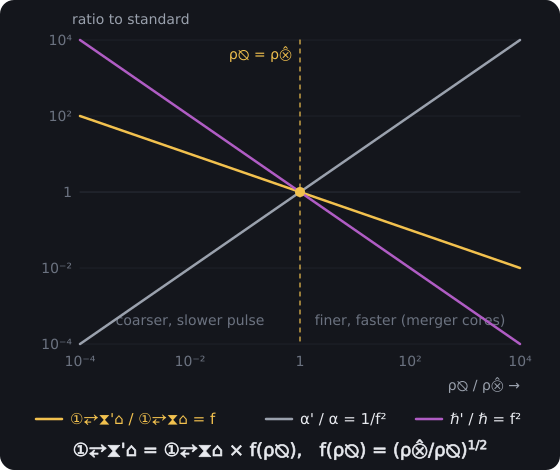
Density-Dependent Time. A universe's Planck time scales with the density of the collapse that formed it, ①⥂⧗'⌂ = ①⥂⧗♁ × f(ρ⦰) with f(ρ⦰) = (ρ⨶/ρ⦰)^(1/2). Here ρ⨶ is the parent's Planck density: a single collapse stays below it and pulses slower, and only a merger-compressed core gives a finer, faster pulse, never below ℨ. With it, α' = α/f² if the charge is unchanged (how α scales is open, Part 1.6) and ℏ' = ℏ × f², while G' = G × (𝒞→'/𝒞→)⁵ stays at G on the ladder; all three equal their standard values at ρ⦰ = ρ⨶.
9.2 Testable Predictions
- Cosmic Microwave Background Temperature Anisotropies: exhibiting density-dependent amplitude variations across sky regions following f(ρ⦰) scaling relationships, detectable with sensitivity better than 10⁻⁷ through multi-frequency cross-correlation analysis revealing systematic spatial patterns.
- Fine Structure Constant Stability: BPT predicts Δα/α = 0 and ΔG/G = 0 across our universe; differences arise only between universes (Part 2.5); statistical analysis of quasar absorption line multiplets across cosmic time is the test.
- Large-Scale Structure Anisotropies: reflecting temporal resolution gradients through correlated galaxy distribution patterns and void geometries in surveys covering volumes greater than (10² Mpc)³, measurable via two-point correlation function deviations from isotropic predictions.
- Gravitational Wave Frequency Signatures: from Null Well Collapses producing characteristic spectral features at frequencies f ∝ 1/①⥂⧗'⌂, detectable by future space-based observatories with strain sensitivity better than 10⁻²¹ at millihertz frequencies.
- Multi-Generational Genealogy Correlations: in cosmic void and filament structures following inheritance scaling relationships across cosmic generations, traceable through statistical analysis of hierarchical structure formation patterns over multiple redshift epochs.
- Fundamental Constant Correlations: between G' and α' measurements indicating common emergence origins from shared collapse density histories, quantifiable through cross-correlation analysis of precision measurements across different cosmic domains.
These predictions could help establish a framework for understanding time as variable-resolution computational substrate rather than uniform background. Binary Pulse Theory's density-dependent temporal resolution offers an account of why Planck time has its specific value while opening new possibilities for computational cosmology and temporal engineering.